Week 3 - Solving second order ODEs
- SOLVING THE SECOND ORDER ODE PROBLEM BY PENDULUM
MAIN FROMULA :-
here : b = damping coefficient i
m = mass of the ball in kg
g = gravity in m/s2
l = length of pendulum in m
% [ dtheta2_dt = -(b/m)*theta2 - (g/l)*sin(theta1) ] equatiion-2 to solve ode
%main function of the ode
function  [dtheta_dt] = ode_func(t,theta, b,l,m,g)
theta1 =theta(1)
theta2 = theta(2)
dtheta1_dt = theta2;
dtheta2_dt = -(b/m)*theta2 - (g/l)*sin(theta1);
dtheta_dt = [dtheta1_dt; dtheta2_dt];
end
%main function of ode screenshot :
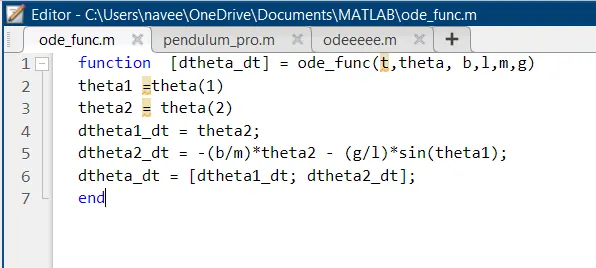
%for above excution check the below program file "ode_func"
% main progarm for pendulum :
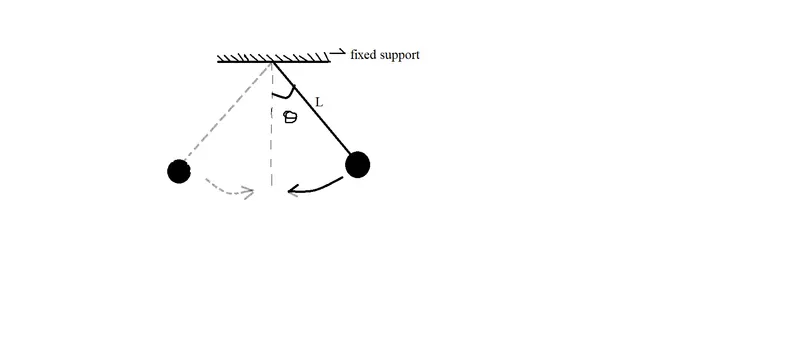
%solving 2nd order ode equations in pendulum motion


clear all
close all
clc

%inputs

m = 1  %mass of body
l = 1  %length
g = 9.81 %gravity
b = 0.05 %damping

%intial condition

theta_0 = [0;3]; %intial condition ; velocity
%time for pendulum motion
t_span = linspace(0,20,300);  %time value(intial,time in sec,values)

%solving ODE

[t, results] = ode45(@(t,theta) ode_func(t,theta, b,l,m,g),t_span,theta_0);

figure(1)
%plotting the results of the pendulum
plot(t,results(:,1));
hold on
plot(t,results(:,2));
xlabel('time')
ylabel('plot')
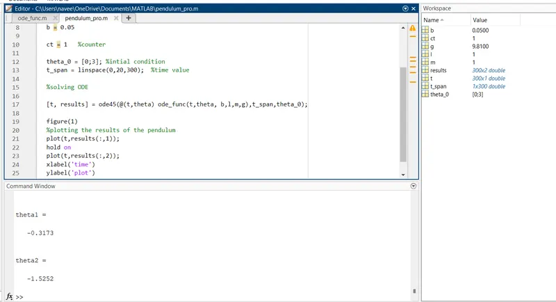
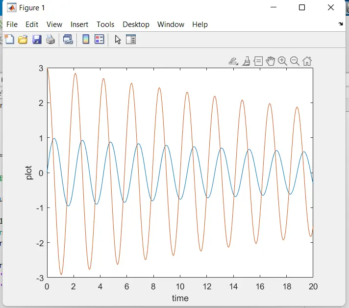
%plot for pendulum motion at the given time .
%for above the excution check the file below "pendulum_pro"
% Creating a program to animate the pendulum motion:
%given inputs
L=1 metre,
m=1 kg,
b=0.05.
g=9.81 m/s2.
Simulate :-
the motion between 0-20 sec
angular_displacement=0
angular velocity=3 rad/sec at time t=0.
%solving ode program to solve pendulum motion


clear all
close all
clc

%INPUTS
m = 1  %mass of body
l = 1   %length of ball
g = 9.81 %gravity in m/s2
b = 0.05 %damping co efficient

ct = 1   %counter

% inital condition
theta_0 = [0;3]; %[intial;velocity]
%time taken to pendulum

t_span = linspace(0,20,300); %(intial,time, value)

%solving ode function

[t, results] = ode45(@(t,theta) ode_func(t,theta, b,l,m,g),t_span,theta_0);

figure(1)
plot(t,results(:,1));
hold on
plot(t,results(:,2));
xlabel('time')
ylabel('plot')

%writing a animation program to pendulum

theta1 = results(:,1);
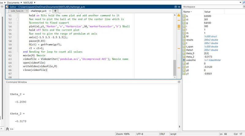
for i = 1:length(theta1) % taking for loop
    theta_2 = theta1(i)

    x0 = 0; %starting value at x
    y0 = 0; %starting value at y

    x1 = l*sin(theta_2);  %ending of x value
    y1 = -l*cos(theta_2); %ending of y value
    %the above negative sign '-' uses because the pendulum motions both
    %postive and negative
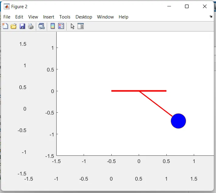
    figure(2)
    % we need to plot the fixed support to motion of pendulum
    plot([-0.5 0.5],[0 0],'linewidth',3,'color','r') %fixed support line
    hold on %its hold the same plot and add another command to it
    %wec need to plot the center line between fixed support and ball
    plot([x0 x1],[y0  y1],'linewidth',2,'color','r') %center line
    hold on %its hold the same plot and add another command to it
    %we need to plot the ball at the end of the center line which is
    %connected to fixed support
    plot(x1,y1,'Marker','o','Markersize',30,'markerfacecolor','b') %ball
    hold off %its end the current plot
    %we need to give the range of pendulum at axis
    axis([-1.5 1.5 -1.5 1.5]);
    pause(0.03)
    M(ct) = getframe(gcf);
    ct = ct+1;
end %ending for loop to count all values
movie(M) %movie
videofile = VideoWriter('pendulum.avi','Uncompressed AVI'); %movie name
open(videofile)
writeVideo(videofile,M)
close(videofile)
%screenshot for progarm
%screenshot for pendulum
% for above program excution check the below program file "challenge_p'
%for the above pendulum motion video click the below link:-