Week 3 - Solving second order ODEs

AIM: To write a program to solve the ordinary diffrential equation of a simple pendulum and simulating the oscilation of the pendulum.

PRE-REQUISITE KNOWLEDGE: A pendulum is a weight suspended from a pivot so that it can swing freely. When a pendulum is displased from its initial position, the bob (mass) is subjected to a restoring force due to gravity. When the bob is released from a desired position, due to restoring force the bob is caused to oscilate about to equilibrium position. The time for one complete cycle, a left and a right swing is called the Period.

GOVERNING EQUATION:

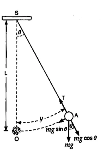
Taking moments of all the forces about the pivot point, we get

`-mgsintheta xx l = I ddottheta`

`ml^2 ddottheta + mgsintheta=0`

`ddottheta+g/lsintheta=0 rarr eq.1`

if damping is taken into consideration then eq.1 becomes

`ddottheta+b/m+g/lsintheta=0`

where,

b = damping coefficient

g = accelaration due to gravity

m = mass of the bob

l = length of the string

CALCULATIONS: let, `theta=thetaunderset(1)() rarr eq.1`

and `(d theta)/(d t)=(d thetaunderset(1)())/(d t)=thetaunderset(2)() rarr eq.2`

then, `(d^2 theta)/(dt)=(d^2 thetaunderset(1)())/dt^2=(d thetaunderset(2)())/(dt)`

we know that, `(d^2 theta)/dt+b/m(d theta)/(dt)+g/lsin(theta)=0`

by substituting eq.1 and eq.2, we get, `(d^2 thetaunderset(1)())/dt^2+b/m(d thetaunderset(1)())/(dt)+g/lsinthetaunderset(1)()=0`

`(d thetaunderset(2)())/(dt)+b/mthetaunderset(2)()+g/lsinthetaunderset(1)()=0`

first ODE, `=> (d thetaunderset(1)())/dt=thetaunderset(2)`

second ODE, `=>(d thetaunderset(2)())/dt=-b/mthetaunderset(2)()-g/lsinthetaunderset(1)()`

writing both the ODEs in matrix form,

`d/dt[[thetaunderset(1)()],[thetaunderset(2)()]]=[[thetaunderset(2)()],[(-b/mthetaunderset(2)()-g/lsinthetaunderset(1)())]]`

CODE: This code is splitted into two codes.

Function Code: The purpose of this code is to store the differential equations which are needed to be numerically integrated using the built-in MATLAB ODE solvers.

% function code
% save as ode_func.m

function [dtheta_dt] = ode_func(t, theta, b, g, l, m)
         theta = theta(1)
         theta = theta(2)
         dtheta1_dt = theta2; % first ODE 
         dtheta2_dt = -(b/m)*theta2-(g/l)*sin(theta1); % second ODE
         dtheta_dt = [dtheta1_dt;dtheta2_dt]; % first & second ODEs written in matrix form
end

Main Code: To solve ordinary differential equation of a simple pendulum and simulating its motion.

%code to solve the ordinary differential equation of a simple pendulum and simulating its motion
%save as ode_main.m

clear all 
close all
clc

% given inputs
b = 0.05; %damping coefficient
g = 9.81; %accelaration due to gravity in m/s^2
l = 1; %length of the string in metre
m = 1; %mass of the bob attached to the string in kg

%initial conditon 
theta_0 = [0,3]; %[initail angular displacement, final angular displacement]

%time points
t_span = linspace(0,20,400);

%solve ODE
[t, results] = ode45(@(t, theta) ode_func(t, theta, b, g, l, m), t_span, theta_0);

%plotting
plot(t, results(:,1)) % time vs angular displacement
hold on % to freeze the previous plot
plot(t, results(:,2)) % time vs angular velocity plot
ylabel('Plot') % y-axis label
xlabel('Time') % x-axis label
legend('Angular Displacement','Angular Velocity') % to distinguish b/w the waves
grid on

%animation
figure(2)
ct = 1;
for i= 1:length(t_span)
    % pivot cooordinates
    x0 = 0;
    y0 = 0;
    
    % free end coordinates
    x1 = l*sin(results(i,1));
    y1 = -l*cos(results(i,1));
  
    % horizontal line to which the pivot is fixed
    plot([-0.5,0.5],[0,0],'linewidth',3,'color','black')
    hold on

    %string
    plot([x0,x1],[y0,y1],'linewidth',2,'color','blue')

    % mass or the bob at the free end
    plot(x1,y1,'marker','O','markersize',15,'markerfacecolor','red')
    hold off

    %adjusting the axis
    axis([-1,1,-1.5,0.5])

    % pausing the frame 
    pause(0.005)
    
    % storing each plot as a frame in an array M
    M(ct) = getframe(gcf);
    ct = ct + 1;
end

% playing the frames as movie
movie(M)

% creation of video file with format
V = VideoWriter('Simple_Pendulum.avi','Uncompressed AVI')

%opening videofile 
open(V)

% writing the opened video file 
writeVideo(V,M)

% closing the video file
close(V) 

ode45 SYNTAX EXPLANATION:

ode45 uses 4th order Runge-Kutta numerical method. The syntax goes as follows.

[t, results] = ode45@((t, theta) ode_func(t, theta, b, g, l, m), t_span, theta_0)

[t, results]`rarr`stores the outputs of anonymous function

ode45@(t,theta)`rarr`is an in-built MATLAB function which is a function of (t,theta) which is been defined here

ode_func(t, theta, b, g, l, m) `rarr`predefined function containing first order ODE which has to be integrated

t_span, theta_0`rarr`first term provides the limits of integration and the second term provides the initial necessary conditions

OUTPUT:

Plot:

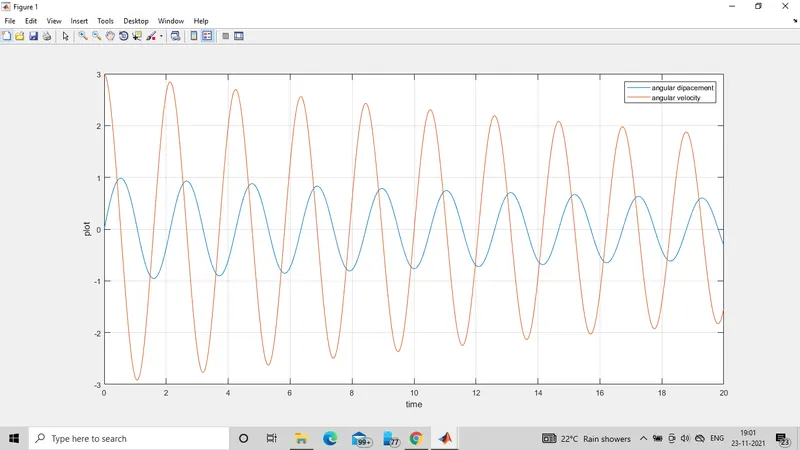
• From the above plot we can clearly see that the angular velocity starts from 3rad/s & angular displacement starts from 0
• After some time both the waves meet at zero this is due to damping which is provided by air.

YouTube Link: https://youtu.be/1vpoIUUolvQ

ERRORS: had made a typo error in simulation of the simple pendulum to which the bob was oscilating in linearly in y-direction