Project 2 - Rankine cycle Simulator
AIM: To create a Rankine Cycle Simulator using Matlab.
PRE-REQUISITE KNOWLEDGE:
Rankine cycle describes the performance of the steam turbine systems through the theoretical principle. The Rankine cycle is an idealized thermodynamic cycle of a constant pressure heat engine that converts part of heat into mechanical work. In this cycle, the heat is supplied externally to a closed loop which uses water as the working fluid. The working fluid in the Rankine cycle undergoes the phase change from liquid to vapour phase and vice versa.
While many substances could be used as the working fluid in the Rankine cycle, water is usually the fluid of choice due to its favourable properties such as non-toxic and non-reactive. Therefore, all the important parameters of water and steam are tabulated in so called “Steam Tables”.
But here instead of steam table we will be using a function called “XSteam.m” which is similar to the steam table in which the required parameters are obtained from the given user inputs.
In an ideal Rankine cycle, the system executing the cycle undergoes a series of four processes: two isentropic (reversible adiabatic) processes alternated with two isobaric processes:
Rankine Cycle – Ts Diagram
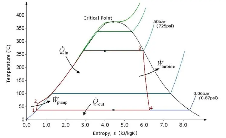
- Isentropic compression (compression in centrifugal pumps) – The liquid condensate is compressed adiabatically from state 1 to state 2 by centrifugal pumps (usually by condensate pumps and then by feed water pumps). The liquid condensate is pumped from the condenser into the higher pressure boiler. In this process, the surroundings work on the fluid, increasing its enthalpy and compressing it (increasing its pressure). On the other hand, the entropy remains unchanged.
- Isobaric heat addition (in a heat exchanger – boiler) – In this phase (between state 2 and state 3), there is a constant-pressure heat transfer to the liquid condensate from an external source since the chamber is open to flow in and out. The feed water (secondary circuit) is heated to the boiling point (2 → 3a) of that fluid and then evaporated in the boiler (3a → 3).
- Isentropic expansion (expansion in a steam turbine) – Steam from the boiler expands adiabatically from state 3 to state 4 in a steam turbine to produce work and then is discharged to the condenser (partially condensed). The steam works on the surroundings (blades of the turbine) and loses an amount of enthalpy equal to the work that leaves the system.
- Isobaric heat rejection (in a heat exchanger) – In this phase, the cycle completes by a constant-pressure process in which heat is rejected from the partially condensed steam. There is heat transfer from the vapour to cooling water flowing in a cooling circuit. The vapour condenses, and the temperature of the cooling water increases.
During a Rankine cycle, the pumps’ work is done on the fluid between states 1 and 2 (isentropic compression). Work is done by the fluid in the turbine between stages 3 and 4 (isentropic expansion). The difference between the work done by the fluid and the work done on the fluid is the network produced by the cycle, and it corresponds to the area enclosed by the cycle curve (in the pV diagram). The working fluid in a Rankine cycle follows a closed loop and is reused constantly.
% RANKINE CYCLE SIMULATION

clear all
close all
clc

% printing the heading and cycle process names
fprintf('***RANKINE CYCLE SIMULATION***\n\n');
fprintf('1-2 : Isentropic Compression\n');
fprintf('2-3 : Constant Pressure Heat Addition\n');
fprintf('3-4 : Isentropic Expansion\n');
fprintf('4-1 : Constant Pressure Heat Rejection\n\n');

%taking the user inputs
t1 = input('Enter turbine inlet temprature (in Deg. C) : ');
p1 = input('Enter turbine inlet pressure (in bar) : ');
p2 = input('Enter turbine outlet pressure (in bar) : ');

%finding specific pressure of the Cp
%saturated liquid and vapour

Cp1_V = XSteam('CpV_p',p1);
Cp1_L = XSteam('CpL_p',p1);
Cp2_V = XSteam('CpV_p',p2);
Cp2_L = XSteam('CpL_p',p2);

%saturation temprature at p1 and p2
Tsat_P1 = XSteam('Tsat_p',p1);
Tsat_P2 = XSteam('Tsat_p',p2);

%Calculating Enthalpy (KJ/Kg) & Entropy (KJ/Kg.K) at saturation points
%Fnding saturated vapour enthalpy (Hg) and entropy (Sg) at State-1 (boiler out)
Hg_1 = XSteam('hV_p',p1);
Sg_1 = XSteam('sV_p',p1);

%Fnding saturated vapour enthalpy (Hg) and entropy (Sg) at State-2 (turbine out)
Hg_2 = XSteam('hV_p',p2);
Sg_2 = XSteam('sV_p',p2);

%Fnding saturated liquid vapour enthalpy (Hg) and entropy (Sg) at State-3 (condensor out)
Hf_1 = XSteam('hL_p',p1);
Sf_1 = XSteam('sL_p',p1);

%Finding saturated liquid vapour enthalpy (Hg) and entropy (Sg) at State-4 (pump out)
Hf_2 = XSteam('hL_p',p2);
Sf_2 = XSteam('sL_p',p2);

%Calculating properties at State-1
fprintf('\nAT STATE POINT - 1 \n');
fprintf('P1 = %0.2f bar \n',p1);
fprintf('T1 = %0.2f deg. C \n',t1);
h1 =  XSteam('h_pT',p1,t1); %enthalpy of superheated water vapour at teh exit of the boiler
fprintf('H1 = %0.2f KJ/Kg \n',h1);
s1 = XSteam('s_pT',p1,t1);
fprintf('S1 = %0.2f KJ/Kg.K \n\n',s1);

%Calculating properties at State-2
fprintf('AT STATE POINT-2\n');
fprintf('P2 = %0.2f bar\n',p2);
s2 = s1; %entropy at state 1 & 2 dosen't change
fprintf('S2 = %0.2f KJ/Kg.K \n',s2);
%calculating dryness fraction X
%dryness fraction at state-2 i.e., x2
if s2<=Sg_2
    x2 = (s2-Sf_2)/(Sg_2-Sf_2);
else
    x2 = 1;
end
fprintf('X2 = %0.2f \n', x2);
%finding t2 at dryness fraction x2
if x2 < 1
    t2 = Tsat_P2; %temprature inside the turbine drops
else
    %s2 = Sg_2 + Cp2_V*log((t2/Tsat_P2))
    t2 = ((Tsat_P2+273.15)*exp((s2-Sg_2)/(Cp2_V)))-273.15;
end
fprintf('T2 = %0.2f deg. C \n',t2);
%finding enthalpy, h2 using dryness fraction x2
if x2 < 1
    h2 = Hf_2 + x2*(Hg_2-Hf_2); %enthalpy of wet steam at turbine exit or condensor inlet
else
    h2 = XSteam('h_pT',p2,t2);
end
fprintf('H2 = %0.2f KJ/Kg \n\n',h2);

%Calculating properties at State-3
fprintf('AT STATE POINT-3 \n');
p3 = p2; %pressure of fluid is same at turbine &condensor outlet
fprintf('P3 = %0.2f bar \n',p3);
t3 = Tsat_P2; %since no sub-coooling is expected
fprintf('T3 =  %0.2f deg. C \n',t3);
v3 = XSteam('vL_p',p3);
h3 = Hf_2; %enthalpy of water at condensor outlet
fprintf('H3 = %0.2f KJ/Kg \n',h3);
s3 = Sf_2; %phase transission from vapuor to liquid
fprintf('S3 = %0.2f KJ/Kg.K \n\n',s3);

%Calculating properties at State-4
fprintf('AT STATE POINT-4 \n');
p4 = p1;
fprintf('P4 = %0.2f bar \n',p4);
s4 = s3; %since the entropy of the liquid dont change while pumping
fprintf('S4 = %0.2f KJ/Kg.K \n',s4);
%work done by pump (Wp)
Wp = v3*(p4-p3)*100;
h4 = Wp +h3; %enthalpy of water at rhe boiler inlet i.e., at the pump outlet
fprintf('H4 = %0.2f KJ/Kg \n',h4);
t4 = ((Tsat_P1 + 273.15)/(exp((Sf_1-s4)/(Cp1_L))))-273.15;
fprintf('T4 = %0.2f deg. C \n\n',t4);

%calculating the workdone, Heat input, Specific Steam Consumption &
%Efficiency
%workdone by the turbine, Wt
Wt = h1 - h2;
fprintf('Workdone by the Turbine = %0.2f KJ/Kg \n', Wt);
fprintf('Workdone by the Pump = %0.2f KJ/Kg \n', Wp);

%net work done = Wnet
Wnet = Wt - Wp;
fprintf('Net Work Done = %0.2f \n', Wnet);

%heat of the fluid after saturation is Qin
Qin = h1 - h4;
fprintf('Heat of the Fluid before Expansion = %0.2f KJ \n', Qin);

%thermal efficiency of the Rankine Cycle
Eff_thermal = (Wnet/Qin)*100;
fprintf('Thermal Efficiency of the cycle = %0.2f',Eff_thermal); disp('%');

%Rankine Cycle Efficiency
Eff_Rankine = ((h1-h2)/(h1-Hf_2))*100;
fprintf('Rankine Efficiency of the cycle = %0.2f',Eff_Rankine); disp('%');

%Specific Steam Consumption of the Turbine (SSC)
SSC = 3600/Wt;
fprintf('Specific Steam Consumption = %0.2f Kg/KWhr \n', SSC);

%Back Work Ratio (BWR)
BWR = Wnet/Wt;
fprintf('Back Work Ratio = %0.2f \n',BWR);
fprintf('***END*** \n');

%calculating the plotting points fot saturation liquid and vapour line
temp = linspace(1,t1,1000);
for i = 1:length(temp)
    H_L(i) = XSteam('hL_T',temp(i));
    H_V(i) = XSteam('hV_T',temp(i));
    S_L(i) = XSteam('sL_T',temp(i));
    S_V(i) = XSteam('sV_T',temp(i));
end

%PLOTTING
%plotting T-S & H-S Diagrams
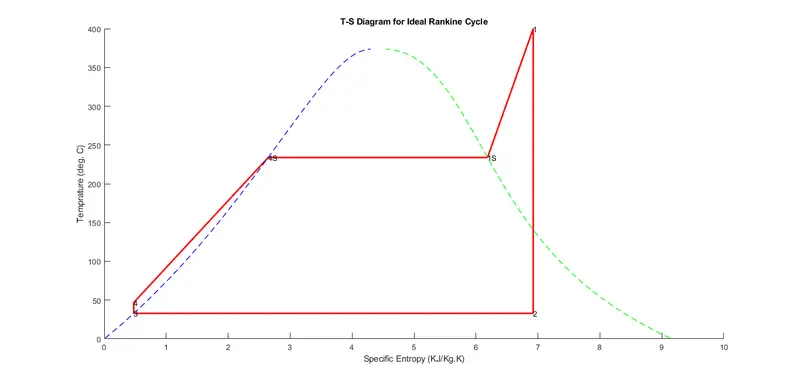
%plotting T-S Diagram
figure(1)
hold on
plot([s1 s2], [t1 t2],'r','linewidth',2);
plot([s2 s3], [t2 t3],'r','linewidth',2);
plot([s3 s4], [t3 t4],'r','linewidth',2);
plot([s4 Sf_1], [t4 Tsat_P1],'r','linewidth',2);
plot([Sf_1 Sg_1], [Tsat_P1 Tsat_P1],'r','linewidth',2);
plot([Sg_1 s1], [Tsat_P1 t1],'r','linewidth',2);
text(s1,t1,'1');
text(s2,t2,'2');
text(s3,t3,'3');
text(s4,t4,'4');
text(Sf_1,Tsat_P1,'4S');
text(Sg_1,Tsat_P1,'1S');
plot(S_L,temp,'b','linestyle','--','linewidth',1);
plot(S_V,temp,'g','linestyle','--','linewidth',1);
title('T-S Diagram for Ideal Rankine Cycle');
xlabel('Specific Entropy (KJ/Kg.K)');
ylabel('Temprature (deg. C)');

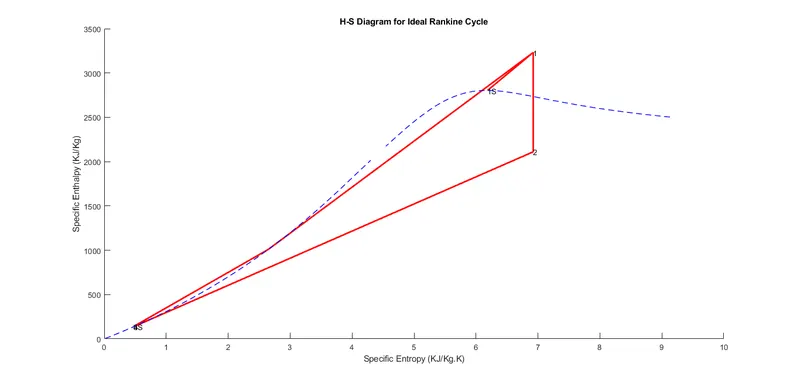
%plotting H-S Diagram
figure(2)
hold on
plot([s1 s2], [h1 h2],'r','linewidth',2);
plot([s2 s3], [h2 h3],'r','linewidth',2);
plot([s3 s4], [h3 h4],'r','linewidth',2);
plot([s4 Sf_1], [h4 Hf_1],'r','linewidth',2);
plot([Sf_1 s1], [Hf_1 h1],'r','linewidth',2);
plot([Sg_1 s1], [Hg_1 h1],'r','linewidth',2);
text(s1,h1,'1');
text(s2,h2,'2');
text(s3,h3,'3');
text(s4,h4,'4');
text(Sf_2,Hf_2,'4S');
text(Sg_1,Hg_1,'1S');
plot(S_L, H_L,'b','linestyle','--','linewidth',1);
plot(S_V, H_V,'b','linestyle','--','linewidth',1);
title('H-S Diagram for Ideal Rankine Cycle');
xlabel('Specific Entropy (KJ/Kg.K)');
ylabel('Specific Enthalpy (KJ/Kg)');
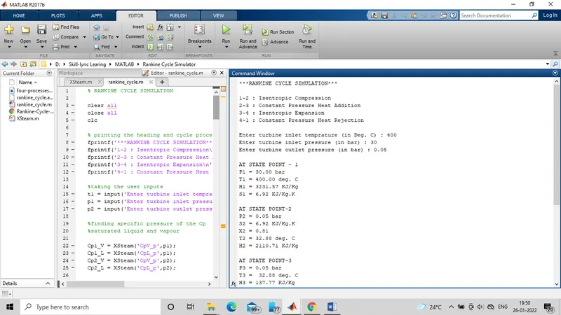
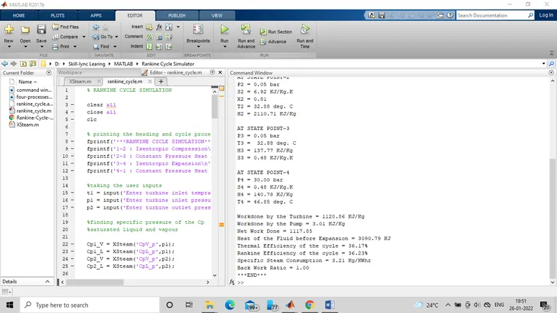
RESULTS :
***RANKINE CYCLE SIMULATION***

1-2 : Isentropic Compression
2-3 : Constant Pressure Heat Addition
3-4 : Isentropic Expansion
4-1 : Constant Pressure Heat Rejection

Enter turbine inlet temprature (in Deg. C) : 400
Enter turbine inlet pressure (in bar) : 30
Enter turbine outlet pressure (in bar) : 0.05

AT STATE POINT - 1
P1 = 30.00 bar
T1 = 400.00 deg. C
H1 = 3231.57 KJ/Kg
S1 = 6.92 KJ/Kg.K

AT STATE POINT-2
P2 = 0.05 bar
S2 = 6.92 KJ/Kg.K
X2 = 0.81
T2 = 32.88 deg. C
H2 = 2110.71 KJ/Kg

AT STATE POINT-3
P3 = 0.05 bar
T3 =  32.88 deg. C
H3 = 137.77 KJ/Kg
S3 = 0.48 KJ/Kg.K

AT STATE POINT-4
P4 = 30.00 bar
S4 = 0.48 KJ/Kg.K
H4 = 140.78 KJ/Kg
T4 = 46.85 deg. C

Workdone by the Turbine = 1120.86 KJ/Kg
Workdone by the Pump = 3.01 KJ/Kg
Net Work Done = 1117.85
Heat of the Fluid before Expansion = 3090.79 KJ
Thermal Efficiency of the cycle = 36.17%
Rankine Efficiency of the cycle = 36.23%
Specific Steam Consumption = 3.21 Kg/KWhr
Back Work Ratio = 1.00
***END***
>> 
REFERENCES :