Week 3 - Solving second order ODEs

Chanllenge Title :- Solving  simple pendulum equation solution with  second order ODEs 

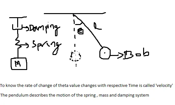
Explanation:- To determine the different position of the pendulum bob and to know the damping frequency 

Formulae for the Second order Damping Equation

`d^2theta/dt^2 + (b/m)*d(theta)/dt + (g/l)*sin(theta)=0`

Where as,

b= damping coeffiecent

g= gravity velocity meters per second 9.81 

l= lenght of the pendulum in meters

m= mass of the pendulum in kgs

Theta = is the Dependent variable having the intial  displacement and  velocity  

t = is the independent variable i.e time span  repersented in one row X  n columns

To solve the second order derivatives  in matlab we can use ODE45  in bulid command

ODE45 means integrates the system of differential equations with respective the defining the function for the dependent variable intial displacement,velocity and Independent variable for time span

After Derivating, the results  can be plots with respective time and result columns

We can create and make animation for the pendulum bob using the movie option in matlab

Subplot:- In this subplot command we are going to divided the graph into required region to show the output plots and animations in single window

Code description:-

clear all
close all
clc
b=0.05;%damping coeffiecent for the bob
g=9.81; %meters/sec
l=1; % meters
m=0.1; % kgs
theta_0=[0;5]; % intial conditons displacment position and velocity 
t_span=linspace(1,20,500); % time span in x-axies
theta_function = @(t,theta) [theta(2);-(b/m)*theta(2)-(g/l)*sin(theta(1))];
%theta_function = @(t,theta) pendulum_function(t,theta,b,m,l,g)
[t,result] = ode45( theta_function , t_span , theta_0 ); 
% t and results are the vectors
subplot (5,4,[13,14,17,18]);
%subplot:- In this subplot command we are going to divided the graph into 
% required region to show the output plots and animations in single window
plot(t, result(:,1),'color','b');
hold on;
plot (t,result(:,2),'color','r');
hold off;
plot(t,result);
subplot(5,4,[15,16,19,20]);
plot(result(:,1),result(:,2));
xlabel('poistion Radians'); %displace the name on x-axies
ylabel('Angular velocity'); %displace the name on y-axies
ct=1; % it used to collect all  the for loop increments to get the
%animation and plot of the required bob
for i= 1:length(result(:,1))
    x0=0;
    y0=0;
    x1=l*sin(result(i,1)); % using trigonmetry formulae
    y1=-l*cos(result(i,1));% using trigonmetry formulae
    % using trigonmetry formulae we can determine the x-cos and y-sin
    % poistions
    subplot(5,4,[1,2,3,4,5,6,7,8,9,10,11,12]);
    xelemtns(ct)= x1;
    yelements(ct)= y1;
    plot([-1,1],[0,0], 'linewidth', 3 , 'color' , 'k')
    line([x0,x1],[y0,y1] ,  'linewidth', 4 , 'color', 'b')
    hold on;
    plot(x1,y1, '-O','markers',20,'markerfacecolor','r');
    grid on; 
    axis([-1.5 1.5 -1.5 0.5])
    pause(0.003)
    hold off;
   %Text = sprintf('pendulum%d.png',ct);
   %saveas(1,Text);
   M(ct)=getframe(gcf);
   ct=ct+1;
end
Videofile= VideoWriter('pendulum_bob.avi'); 
% write the video means create a file of M(ct)
open(Videofile) % open the file to save
writeVideo(Videofile,M) % writing the kinematic animation links in to veidofile
close(Videofile)

 Outputs:-

all the required output  code, plots and animation are attached below