Week 3 - Solving second order ODEs

Aim: To write a program to solve the seconde order ODE for the motion of a simple pendulum and tp plot the angular displacement and angular velocity with respect to time.

Theory:

Let

theta=theta1

dtheta1/dt=theta2

dtheta^2/dt=dtheta2/dt

Main code explanation

The input variable are given

b=0.05; % Damping Co efficient(Ns/m)
g=9.81; % Acceleration due to gravity(m/s^2)
l=1; % Length of the string (m)
m=1; % Mass of the bob of pendulum

An array theta_0 is created with initial values of displacement and velocity

theta_0=[0;3]; % Column vector with initial displacement as 0 as initial velocity 3

An array t_span is created with 500 values of time span between 0 and 20 seconds.

t_span=linspace(0,20,500);

The second order ODE is solved by calling the function

[t,results]=ode45(@(t,theta) ode_function(t,theta,b,g,l,m),t_span,theta_0);

******

Function code

function[dtheta_dt]=ode_function(t,theta,b,g,l,m)
theta1=theta(1)
theta2=theta(2)
dtheta1_dt=theta2;
dtheta2_dt=-(b/m)*theta2-(g/l)*sin(theta1);
dtheta_dt=[dtheta1_dt;dtheta2_dt];
end

The equation is solved using the above code.

The output is plotted using the plot command.

For creating the animation of the motion of pendulum, for loop is used and loop counter is initiated

The values are stored in theta_1.

The base for pendulum is plotted using command

plot([-3 3],[0 0],'linewidth',3,'color','black')

The string of pendulum is plotted using command

plot([X0 X1],[Y0 Y1],'linewidth',1.5,'color','g')

The bob of pendulum is plotted using command

plot(X1,Y1,'marker','o','MarkerSize',20,MarkerFaceColor='b')

All the frames dre compiled using the command

M(ct)=getframe(gcf);

The animation movie is saved using the command

movie(M)
videofile=VideoWriter('SimplePendulum.avi','Uncompressed AVI')
open(videofile)
writeVideo(videofile,M)
close(videofile)

% Program to solve Second order ODE
clear all 
close all
clc

% Input variables
b=0.05;         % Damping Co efficient(Ns/m)
g=9.81;         % Acceleration due to gravity(m/s^2)
l=1;            % Length of the string (m)
m=1;            % Mass of the bob of pendulum

% Initial codition
theta_0=[0;3];  % Column vector with initial displacement as 0 as initial velocity 3

% Timepoints
t_span=linspace(0,20,500);

% Solve ODE
[t,results]=ode45(@(t,theta) ode_function(t,theta,b,g,l,m),t_span,theta_0);
 
% Plotting
figure(1);
plot(t,results(:,1))
hold on
plot(t,results(:,2))
xlabel('Time')
ylabel('Plot')

% iloop for creating animation of simple pendulum
ct=1;
theta_1=results(:,1);
for i=1:length(theta_1)
%initial values
X0=0;
Y0=0; 
theta_2=theta_1(i);
%initial values
X0=0;
Y0=0;
% Final values
X1=l*sin(theta_2);
Y1=-l*cos(theta_2);
figure(2);
% Plotting Pendulum base
plot([-3 3],[0 0],'linewidth',3,'color','black')
hold on
% Plotting Pendulum string
plot([X0 X1],[Y0 Y1],'linewidth',1.5,'color','g')
% Plotting pendulum bob
plot(X1,Y1,'marker','o','MarkerSize',20,MarkerFaceColor='b')
axis([-3 3 -3 3 ])
pause(0.01)
hold off
M(ct)=getframe(gcf);
ct=ct+1;
end
movie(M)
videofile=VideoWriter('SimplePendulum.avi','Uncompressed AVI')
open(videofile)
writeVideo(videofile,M)
close(videofile)

% Function program to calculated second order ODE
function[dtheta_dt]=ode_function(t,theta,b,g,l,m)
theta1=theta(1)
theta2=theta(2)
dtheta1_dt=theta2;
dtheta2_dt=-(b/m)*theta2-(g/l)*sin(theta1);
dtheta_dt=[dtheta1_dt;dtheta2_dt];
end

Output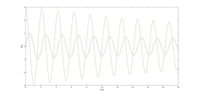

Animation file Youtube link:https://youtu.be/SkSuuNV4FrQ

Errors :Not using the negative sign(-) in the code.

Y1=-l*cos(theta_2);

Other typo errors are cleared while running.