Week 3 - Solving second order ODEs

Aim: To simulate a transient behavior of a simple pendulum by solving second order ODEs using MATLAB.

Objective of the project:

• To write a program that solves the following ODE. This ODE represents the equation of motion of a simple pendulum with Damping.

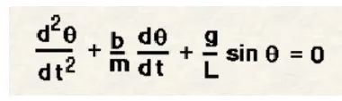
Where

b = damping coefficient(N-m/s)

m = mass of the bob in K.g

g = gravitational acceleration(m/s)

l = length of the string to connect a bob (m)

• The above equation is having a differential power of order 2. To use ode45 solver which uses the simple differential equation to solve The higher order differential equation.

Theoretical Background

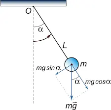
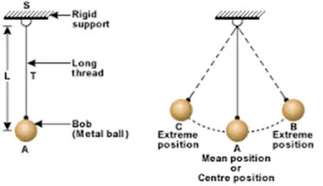
• The Above figure shows idealized pendulum, with a ‘’massless” string or rod of length L and a bob of mass M.
• The dotted circle shows the rest position of the bob. When we give external force it swings back and forth.
• The primary forces like gravitational force that makes it move in the first place and the force exerted by the string to keep it moving along a circular path.
• In addition, it will have a damping force from friction at the pivot or air resistance.
• We will construct a model to describe how the angle theta of the pendulum varies as function of time t.

Matlab code:

clear all
close all 
clc

%inputs
b=0.05;   %damping coefficient
g=9.81;   %gravity(m/s^2)
l=1;       %length of the spring (m)
m=1;      %mass of the bob (kg)

%initial conditions
%initital angular displacent is 0 and angular velocity is 5m/s 
theta_0 = [0;3]

%Time span is the time array
%pendulum oscilltes betweeen o-20 seconds
t_span = linspace(0,20,600)

% solving ODE
[t,results] = ode45(@(t,theta)ode_function(t,theta, b,g,l,m),t_span,theta_0);

%plotting
figure(1)
plot(t,results(:,1))
hold on
plot(t,results(:,2))
title('Damped Harmonic motion of a pendulum')
legend('Angular displacement','angular velocity')
xlabel('time(sec)')
ylabel('plot')

%for loop
%before for loop a counter value is defined
 figure
ct = 1;
for i = 1:length(results(:,1))
    %initial boundary condition
    x0 = 0
    y0= 0
    
    %Defining x and y coordinates
    x1 = l*sin(results(i,1))
    y1 = -l*cos(results(i,1))
    
    %animation
    figure(2)
    plot([-1 1],[0 0],'linewidth',4)
    hold on
    plot([0 0],[-1.5 0.5],'Linestyle','--','color','black')
    plot([x0 x1],[y0 y1],'linewidth',1,'color','b')
    plot(x0,y0,'o','markersize',4,'markerfacecolor',[0.6 0.6 0.6]);
    plot(x1,y1,'o','markersize',20,'markerfacecolor','r')
    title('animation of a pendulum')
    axis([-1.5 1.5 -1.5 1])
    pause(0.03)
    hold off
    M(ct) = getframe(gcf)
    ct = ct+1
end

%animated video
 movie(M)
 videofile = VideoWriter('pendulum_animation.avi');
 open(videofile)
 writeVideo(videofile,M)
 close(videofile)

Ode_func code:

%function program
function [dtheta_dt] = ode_function(t,theta,b,g,l,m)
   
theta1 = theta(1)
theta2 = theta(2)
dtheta1_dt = theta2;
dtheta2_dt = -(b/m)*theta2 - (g/l)*sin(theta1);
dtheta_dt = [dtheta1_dt; dtheta2_dt];
end

Code Explanation:

• Define the input parameters as g = gravity in m/s^2, Length in mm, mass of the ball in k.g , b = damping coefficient
• ode45 solver in Matlab that solves the ordinary or partial differential equations using a numerical method. In this problem the highest order is 2. So we have to take two constant values so that the equation is changed to simple differential equation, to create a ode_func() which will return a column matrix for the solver with the reduced first order equations.
• Provide time limit and initial conditions according to the ode45
• Results contain two separate columns, access the result array to plot the angular velocity and angular displacement.
• Using for loop capture the variation of time and plot the location of pendulum with co-ordinates varying as a Function of angular displacement.
• Create a animation of the pendulum.

Observation:

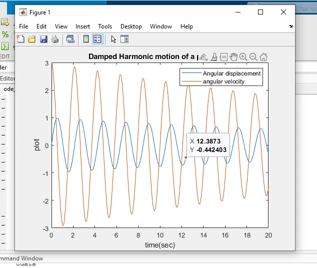
The damped harmonic motion of the pendulum can be observed from the graph where we can observe both the velocity and displacement getting reduced due to damping effect.

Conclusion:

The equation for the simple pendulum is solved and the results is shown in graphical representation. An animation is made for simple pendulum using MATLAB by second order ODE.

Youtube link for the animation of the pendulum:

https://youtu.be/WOvmszg6pWw