Challenge

Week 3 - Solving second order ODEs

AAtharva Choudhari6 Oct 2021

AIM: To simulate the transient behavior of a simple pendulum and to create an animation of its motion.
OBJECTIVE
1. To write a program in Python that solves the second-order ODE corresponding to the motion of a simple
angular displacement and angular velocity wrt time.
2. To create the animation of the motion of pendulum
PROCEDURE
1. At first math, matplotlib, numpy and scipy modules were imported for their various functions.
2. Initial inputs such as b,g,l,m are provided according to data in the question.
3. An array of initial theta was created to define initial angular displacement and initial angular velocity.
4. To solve the second-order ODE, a function named module which stores the above matrix data in it.
5. The given second-order ODE was solved using odeint' command followed by the proper syntax of the calling fun
obtained was used to plot the graph of variation of angular displacement and angular velocity wrt time.
6. Now for creating the animation of the obtained harmonic motion of the pendulum, for loop was used and a loop
initiated, the values of angular position is stored in a separate variable called 'tmp' and is iterated in for loop. In this
of the string of pendulum was fixed and the other end moves according to the solution of the ODE solved.

CODE

#A program for solving second order ODEs and simulate its motion

import math
import matplotlib.pyplot as plt
import numpy as np
from scipy.integrate import odeint

def model(theta,t,b,g,l,m):
	theta1 = theta[0]
	theta2 = theta[1]
	dtheta1_dt = theta2
	dtheta2_dt =  -(b/m)*theta2- (g/l)*math.sin(theta1)
	dtheta_dt = [dtheta1_dt, dtheta2_dt]
	return dtheta_dt

# Inputs
# damping coefficient
b = 0.05
# acceleration due to gravity 
g = 9.81
# length of string 
l =1
#mass of bob 
m = 1
# Initial Conditions
theta_0 = [math.pi/2,0]
#time points
t = np.linspace(0,20,100)

#solve ode 
theta = odeint(model, theta_0,t,args = (b,g,l,m))

# plot results
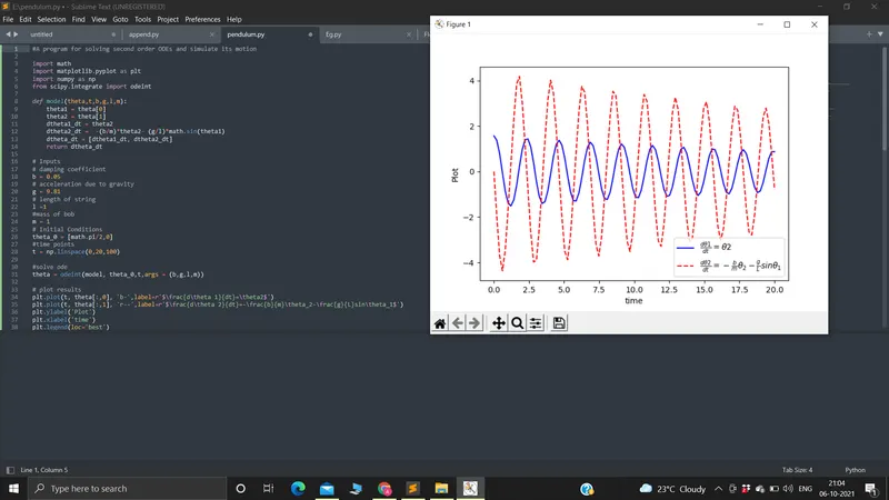
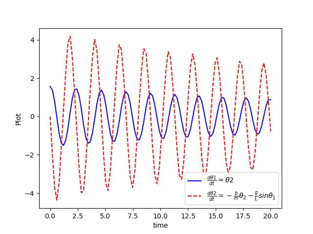
plt.plot(t, theta[:,0], 'b-',label=r'$\frac{d\theta 1}{dt}=\theta2$')
plt.plot(t, theta[:,1], 'r--',label=r'$\frac{d\theta 2}{dt}=-\frac{b}{m}\theta_2-\frac{g}{L}sin\theta_1$')
plt.ylabel('Plot')
plt.xlabel('time')
plt.legend(loc='best')
plt.show()

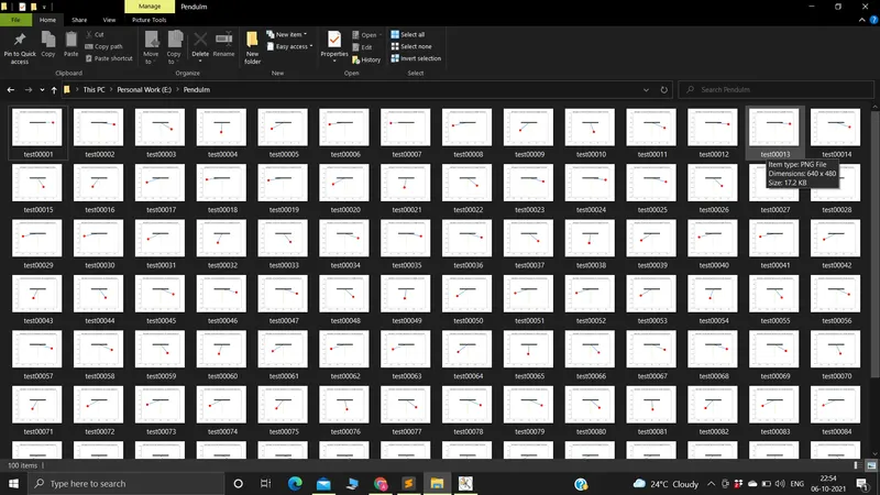
# Iteration using for loop to create animation of motion of pendulum

loop_counter = 1 
tmp = theta[:, 0]
for i in tmp:
	x_start = 0
	y_start = 0
	x_end = 1*math. sin(i)
	y_end = -1*math.cos(i)
	# Plotting fbr animation
	plt. figure()
	# Plotting String of pendulum
	plt.plot ([x_start,x_end],[y_start,y_end],linewidth=3)
	# Plotting Bob of pendulum
	plt.plot (x_end,y_end, 'o', markersize=20, color='r')
	# Plotting the rigid support through which string of pendulum is attached
	plt.plot ([-0.5,0.5],[0,0], linewidth=8, color='k')
	# Plotting hatched vertical line for refernce
	plt.plot([0,0],[0,-1.5],'--',color='y')
	plt.xlim([-1.25,1.25])
	plt.ylim([-2,1])
	plt. title(' Animation of transient behaviour of a Simple Pendulum')
	filename = 'test%05d.png' % loop_counter
	plt.savefig(filename)
	loop_counter = loop_counter + 1

Week 3 - Solving second order ODEs

Ship work like this
in your own course.

Talk to a career counsellor

Ship work like thisin your own course.

Talk to a career counsellor

Ship work like this
in your own course.