Week 3 - Solving second order ODEs

Aim

To write a code to simulate simple pendulum motion

Introduction

In engineering, ODE is used to describe the transient behaviour of a system. A example is a simple pendulum. The following is the second order ode of a simple pendulum. The way the pendulum moves depends on the newtons second law .

Formula

lets say

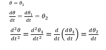
Breaking down Second order ODE into a series of two first order ODE

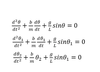
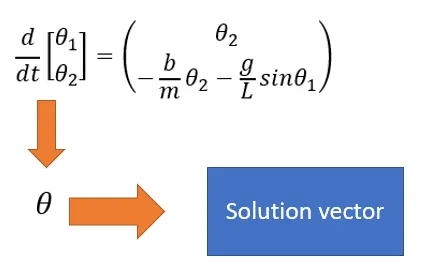
where,

g = gravity in m/s2,

L = length of the pendulum in m,

m = mass of the ball in kg,

b=damping coefficient.

From the figure we can get to know axis which is required for simulation

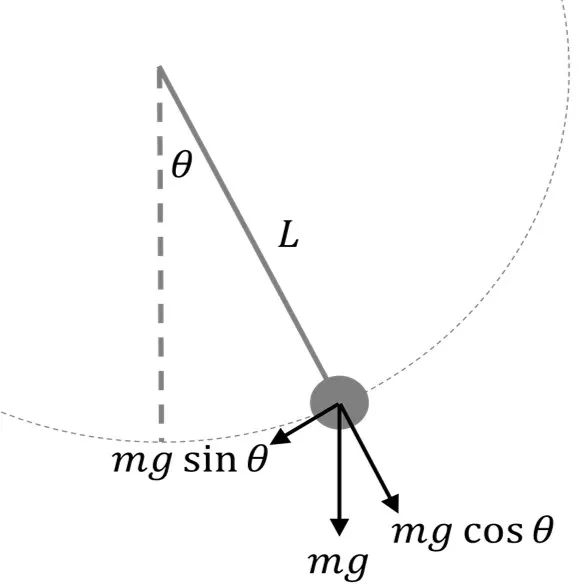
x0=(0)
y0=(0)

x1=-L*cos(θ)
y1=L*sin(θ) or -L*sin(θ)

θ=displacement

Explanation of the code

• clear all (This clears your workspace) ,
• close all(closes all figures) and
• clc (clears the command window).

Inputs
b=.05; damping coefficient.
g=9.81m/s2.; gravity in m/s2,
L=1 m; length of the pendulum in m,
m=0.1 kg; mass of the ball in kg,

Initial condition
theta_0=[0;3] Angular displacement=0,Angular velocity=3 rad/sec

Time points
t_span=linspace(0,20,200) Simulate the motion between 0-20 sec(linspace-Generate linearly spaced vector)

Solve ODE

[t, result] =ode45(@(t,theta)ode_func(t,theta,b,g,L,m),t_span,theta_0)

ode45 is a solver in MATLAB which solves ODEs

@(t,theta)-are values on which the function depends on

ode_func- callin the piece of code.

Plotting
figure(1) Represents the second figure

plot(t, result(:,1)) plots the result of first column
hold on retains plots
plot(t,result(:,2)) plots the result of second column
ylabel('velocity/displacement') Label y-axis
xlabel('time') Label x-axis

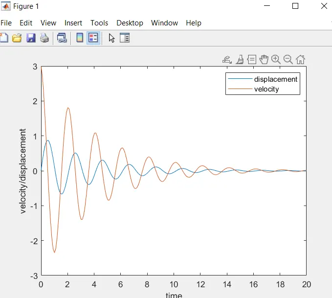
legend('displacement','velocity') MATLAB function creates a legend with descriptive labels for each plotted data series.

ct=1

In computer programming a loop counter is the variable that controls the iterations of a loop and here after each for loop the counter is incrementing.

for i=1:length(result(:,1)) -it represents the length of (i) i,e 1 to 500

• A "For" Loop is used to repeat a specific block of code a known number of times. In hear we are repeating the result of the displacement.

theta=(result(i,1));

In here (i) takes each from 1 to 500 one after the other and (1)represents takes the value of displacement from the result for each values from 1 to 500 and the values is stored in theta.

positions of the links can be decided by this axis points

x0=0
y0=0

x1=L*sin(theta )
y1=-L*cos(theta )

Plotting
figure(2) Represents the second figure

Plot command is used for graphical representation
plot([x0 x1],[y0 y1],[-0.25 0.25],[0 0],'linewidth',3)

plots a line from xo yo to x1 y1

similarly plots the line from -0.25 to 0.25 in x direction and 0 0 in y direction

linewidth thickens the size of the curve or line

hold on retains the figure

plot(x1,y1,'o','MarkerFaceColor','red','markersize',20)

'o'-represents the circle

Markerfacecolor ','red' -color of the circle

'markersize'- sets a size of the marker

hold off

hold off sets the hold state to off so that new plots added to the axes clear existing plots

axis([-1.5 1.5 -1.5 1 ])

Set axis limits and aspect ratios

M(ct)=getframe(gcf);

captures the figure for each counter. (gcf mean get current frame)

ct=ct+1;

In computer programming a loop counter is the variable that controls the iterations of a loop and here after each for loop the counter is incrementing.

end (ending the the for loop)

movie(M)

Play recorded movie frames

videofile= VideoWriter('forward_kinematics.avi' ,'uncompressed AVI');

Use a VideoWriter object to create a video file from an array or MATLAB movie in the name forward_kinematics in a uncompressed manner.

open

opens the specified file

writeVideo(videofile,M)

saves/Write video data to file

close (videofile)

closes the video file

Piece of code which has to be called to the main code

function[dtheta_dt] =ode_func(t,theta,b,g,L,m)

defing a function

Breaking down Second order ODE into a series of two first order ODE
dtheta1_dt= theta(2) -------1

dtheta2_dt=-(b/m)*theta(2)-(g/L)*sin(theta(1))--------2

dtheta_dt=[dtheta1_dt ;dtheta2_dt]--------- column matrix hence ';'
end

Error faced

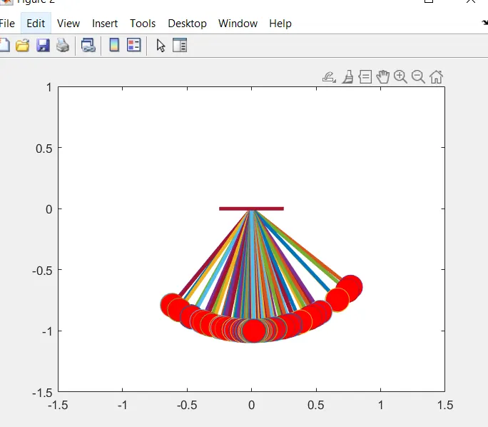
Corrective action taken to fix the error was introducting hold off command

Main Code

clear all
close all
clc
%inputs
b=.05;
g=9.81;
L=1;
m=0.1;

%initial codition
theta_0=[0;3]

%time points
t_span=linspace(0,20,200)

%solve ODE

[t, result] =ode45(@(t,theta)ode_func(t,theta,b,g,L,m),t_span,theta_0)

%plot
figure(1)
plot(t, result(:,1))
hold on
plot(t,result(:,2))
ylabel('velocity/displacement')
xlabel('time')
legend('displacement','velocity') 

ct=1
for i=1:length(result(:,1))
  
   theta=(result(i,1));
       
x0=0
y0=0

x1=L*sin(theta )
y1=-L*cos(theta)




 %plotting
figure(2)
plot([x0 x1],[y0 y1],[-0.25 0.25],[0 0],'linewidth',3)

hold on

plot(x1,y1,'o','MarkerFaceColor','red','markersize',20)
hold off

axis([-1.5 1.5 -1.5 1 ])

M(ct)=getframe(gcf);
ct=ct+1;

    end


%creating animation and saving the file
movie(M)
videofile= VideoWriter('pendulum.avi' ,'uncompressed AVI');
open(videofile)
writeVideo(videofile,M)
close (videofile)

Piece of code which is called to main code

function[dtheta_dt]   =ode_func(t,theta,b,g,L,m)

dtheta1_dt= theta(2)
dtheta2_dt=-(b/m)*theta(2)-(g/L)*sin(theta(1))
dtheta_dt=[dtheta1_dt ;dtheta2_dt]
end

Result

Displacement starts with zero and angular velocity 3 rad/sec. The pendulum comes to rest due to the damping in the span of 20s and it is represented the figure1

click the link below to veiw the animation of the Pendulum

https://drive.google.com/file/d/1usR2md0XlFrrokZEzzyhXtotGD_wTMEO/view?usp=sharing