Week 3 - Solving second order ODEs

AIM:

To write a program that solves the equation of the motion of a simple pendulum with damping.

CONCEPT:

• For a simple pendulum with a damping factor, the equation of simple pendulum is

Where

b = damping coefficient (N-m/s)

m = mass of the bob (kg)

g = gravitational acceleration (m/s)

l = length of the string to connect bob (m)

• The above equation is having a differential power of order 2. To use ode45 solver which is developed on the basis of RK method which uses the simple differential equation to solve the higher order differential equations.

OBJECTIVE:

• By using ode45 solver which is an inbuilt solver in MATLAB. The ode45 solver should require a simple differential equation to solve any kind of higher-order differential equation.
• By taking constants we can solve the higher-order differential equation to a simple ordinary differential equation

SIMPLE PENDULUM:

An ideal pendulum consisting of a point mass suspended by a weightless inextensible perfectly flexible thread and free to vibrate without friction.

The way the pendulum moves depends on newton's 2nd law.

Let us consider

θ = θ1 ------ (1)

dθ/dt = dθ₁/dt = θ₂ ------(2)

d²θ/dt² = dθ₂/dt -------(3)

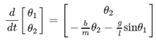
• By using these constants, the second order equation will become as:

dθ₂/dt = -(b/m) * θ₂ – (g/l) * sinθ

• The simple differential equations are written in the form of a matrix

• By using the above equation and the ode45 solver we can animate the simple pendulum in MATLAB by writing a code.

CALLING FUNCTION CODE

%calling function

function [dtheta_dt]=ode_func(t ,theta,b,g,l,m)

theta1=theta(1);
theta2=theta(2);
dtheta1_dt=theta2;

dtheta2_dt= -(b/m)*theta2-(g/l)*sin(theta1);

dtheta_dt=[dtheta1_dt;dtheta2_dt];

end

PROGRAM

clear all
close all
clc

%inputs
%damping coefficient
b=0.05
%length of pendulum in m
l=1
%mass of the ball in kg
m=1
%gravity in m/s^2
g=9.81

%initial condition
theta_0 = [0;5];

t_span = linspace(0,20,200);

% solve ode

[t,results]=ode45(@(t,theta) ode_func(t,theta,b,g,l,m),t_span,theta_0)

figure(1)
plot(t,results(:,1))
hold on
plot(t,results(:,2))
xlabel('time')
ylabel('theta')
legend('angular displacement','angular velocity')

hold off

ct=1;

% fixed coordinates of pendulum

for i=1:length(t)
x0=0;
y0=0;
x1=l*sin(results(i,1));
y1=-l*cos(results(i,1));

% moving coordinates of the pendulum

figure(2)
plot([x0 x1],[y0 y1],'color','r')
hold on
plot([1 -1],[0 0],'color','b')

%plotting of bob

plot(x1,y1,'.','MarkerSize',50)
axis([-1 1 -1 1])
hold off



% create a movie of a simple pendulum

M(ct)=getframe(gcf);
ct=ct+1;
end
movie(M)
videofile = VideoWriter('Pendulum_ODE.avi','uncompressed AVI');
open(videofile)
writeVideo(videofile,M)
close(videofile)

ERRORS:

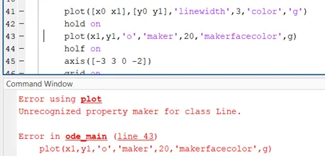
• while using the ‘MarkerFaceColor’ I was not aware of the capital letters of the command to be specified.

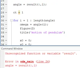
• using the results command, in figure 1 to get the plot the output is stored in results. But using it again to take the input for the motion of the pendulum I have written it as a result which MATLAB showed it as an error.

OUTPUT

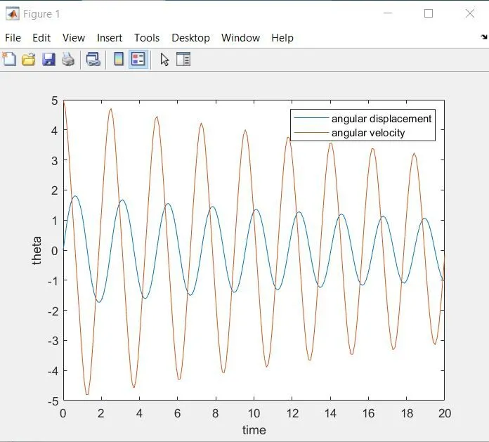
Time vs Angular displacement and Angular velocity :

• The plot explains how the angular velocity and angular displacement is varying with respect to time

• We can observe here how angular velocity and displacement are changing with respect to time.

ANIMATION

CONCLUSION:

• We have animated the simple pendulum using the ode45 solver where the second-order is reduced to a simple differential equation where it is easy to solve the given equation.
• The animation is made using the different points of the bob and the motion of the simple pendulum is created.