Week 3 - Pitot tube
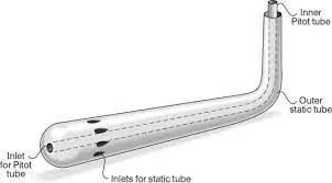
A pitot tube, also known as a pitot probe, is a flow measurement device used to measure fluid flow velocity. The pitot tube was invented by the French engineer Henri Pitot in the early 18th century and was modified to its modern form in the mid-19th century by French scientist Henry Darcy. It is widely used to determine the airspeed of an aircraft, the water speed of a boat, and to measure liquid, air, and gas flow velocities in certain industrial applications. The basic pitot tube consists of a tube pointing directly into the fluid flow. As this tube contains fluid, a pressure can be measured; the moving fluid is brought to rest (stagnates) as there is no outlet to allow flow to continue. This pressure is the stagnation pressure of the fluid, also known as the total pressure or (particularly in aviation) the pitot pressure.
The measured stagnation pressure cannot itself be used to determine the fluid flow velocity (airspeed in aviation). However, Bernoulli's equation states:
- Stagnation pressure = static pressure + dynamic pressure
Which can also be written

Solving that for flow velocity gives

where
 is the flow velocity;
 is the stagnation or total pressure;
 is the static pressure;
 is the fluid density.
The above equation applies only to fluids that can be treated as incompressible. Liquids are treated as incompressible under almost all conditions. Gases under certain conditions can be approximated as incompressible. The dynamic pressure, then, is the difference between the stagnation pressure and the static pressure. The dynamic pressure is then determined using a diaphragm inside an enclosed container. If the air on one side of the diaphragm is at the static pressure, and the other at the stagnation pressure, then the deflection of the diaphragm is proportional to the dynamic pressure.
In aircraft, the static pressure is generally measured using the static ports on the side of the fuselage. The dynamic pressure measurement can be used to determine the indicated airspeed of the aircraft. The diaphragm arrangement described above is typically contained within the airspeed indicator, which converts the dynamic pressure to an airspeed reading employing mechanical levers. Instead of separate pitot and static ports, a pitot-static tube (also called a Prandtl tube) may be employed, which has a second tube coaxial with the pitot tube with holes outside the sides direct airflow, to measure the static pressure.
PITOT STATIC TUBE
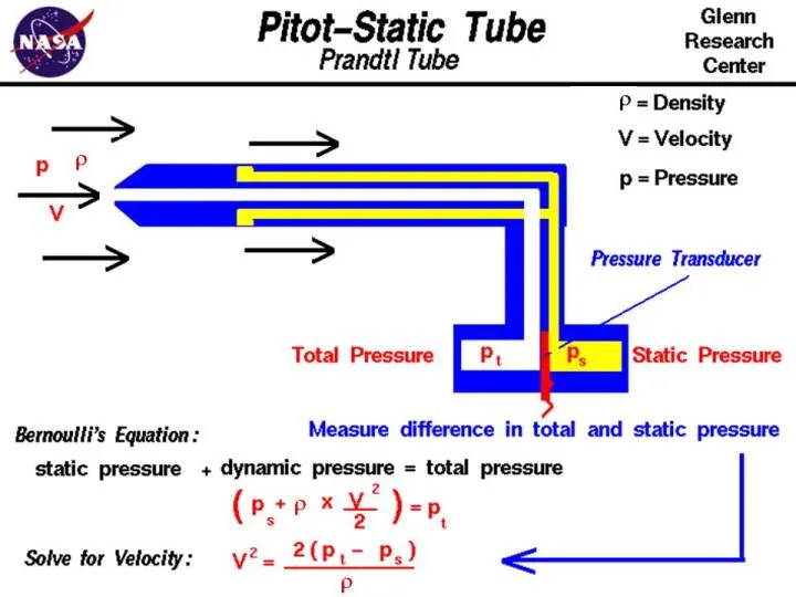
The image shows a schematic drawing of a pitot-static tube. Pitot-Static tubes, which are also called Prandtl tubes, are used on aircraft as speedometers. The actual tube on the aircraft is around 10 inches (25 centimeters) long with a 1/2 inch (1 centimeter) diameter. Several small holes are drilled around the outside of the tube and a center hole is drilled down the axis of the tube. The outside holes are connected to one side of a device called a pressure transducer. The center hole in the tube is kept separate from the outside holes and is connected to the other side of the transducer. The transducer measures the difference in pressure in the two groups of tubes by measuring the strain in a thin element using an electronic strain gauge. The pitot-static tube is mounted on the aircraft, or in a wind tunnel so that the center tube is always pointed in the direction of the flow and the outside holes are perpendicular to the center tube. On some airplanes, the pitot-static tube is put on a longer boom sticking out of the nose of the plane or the wing.
The difference in Static and Total Pressure
Since the outside holes are perpendicular to the direction of flow, these tubes are pressurized by the local random component of the air velocity. The pressure in these tubes is the static pressure (ps) discussed in Bernoulli's equation. However, the center tube is pointed in the direction of travel and is pressurized by both the random and the ordered air velocity. The pressure in this tube is the total pressure (pt) discussed in Bernoulli's equation. The pressure transducer measures the difference in total and static pressure which is the dynamic pressure q.
measurement = `q=pt-ps`
Solve for Velocity
With the difference in pressures measured and knowing the local value of air density from pressure and temperature measurements, we can use Bernoulli's equation to give us the velocity. In the graphic, the Greek symbol rho is used for air density. In this text, we will use the letter r. Bernoulli's equation states that the static pressure plus one-half the density times the velocity V squared is equal to the total pressure.
`ps + .5 * r * V ^2 = pt`
Solving for V:
`V ^2 = 2 * {pt - ps} / r`
`V = sqrt [2*{pt - ps} / r ]`
where sqrt denotes the square root function.
There are some practical limitations to the use of a pitot-static tube:
- If the velocity is low, the difference in pressures is very small and hard to accurately measure with the transducer. Errors in the instrument could be greater than the measurement! So pitot-static tubes don't work very well for very low velocities.
- If the velocity is very high (supersonic), we've violated the assumptions of Bernoulli's equation and the measurement is wrong again. At the front of the tube, a shock wave appears that will change the total pressure. There are corrections for the shock wave that can be applied to allow us to use pitot-static tubes for high-speed aircraft.
- If the tubes become clogged or pinched, the resulting pressures at the transducer are not the total and static pressures of the external flow. The transducer output is then used to calculate a velocity that is not the actual velocity of the flow. Several years ago, there were reports of icing problems occurring on airliner pitot-static probes. Output from the probes was used as part of the auto-pilot and flight control system. The solution to the icing problem was to install heaters on the probes to ensure that the probe was not clogged by ice build-up.
PITOT TUBE SIMULATION [v = 62m/s]
For the simulation part, we are going to import the mesh file directly into the Fluent solver as shown below
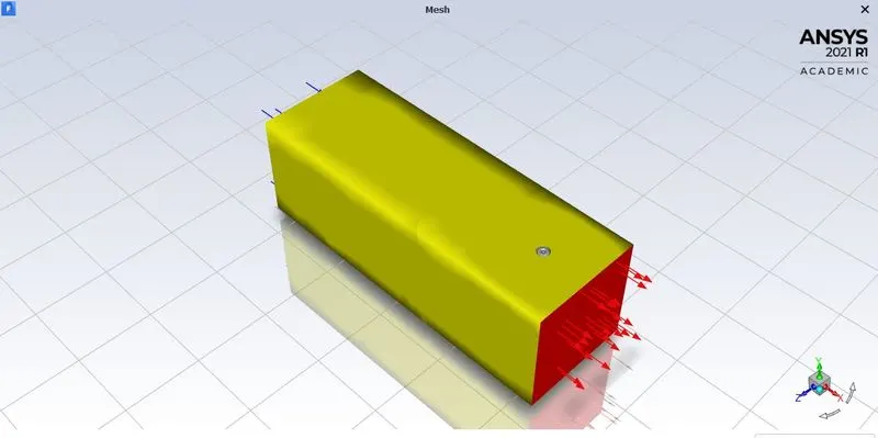
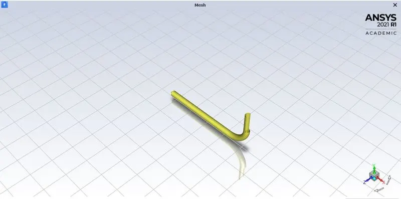
The pitot tube is shown in the fluent solver which will be placed within a enclosure for the flow to take place from inlet of pitot tube towards the outlet to measure the velocity of the fluid stream.
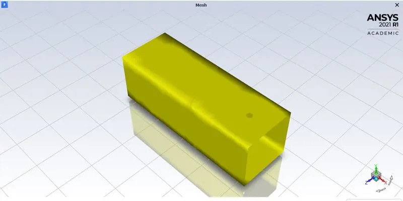
The above image shows the enclosure clearly with holes on the top to measure the static and dynamic pressure.
Setup
The simulation was setup as follows
- Solver - Pressure solver
- Solver Type - Steady
- Viscous - Laminar Flow
- Density = 0.86 `[kg]/m^3`
- Boundary Conditions
Inlet
- Inlet - velocity inlet
- Velocity = 62 m/s
- Pressure = 65780 Pa
Outlet
- Outlet - Pressure Outlet
- Pressure = 65780 Pa
Solution

Results [ V = 62 m/s]
Pressure Contour
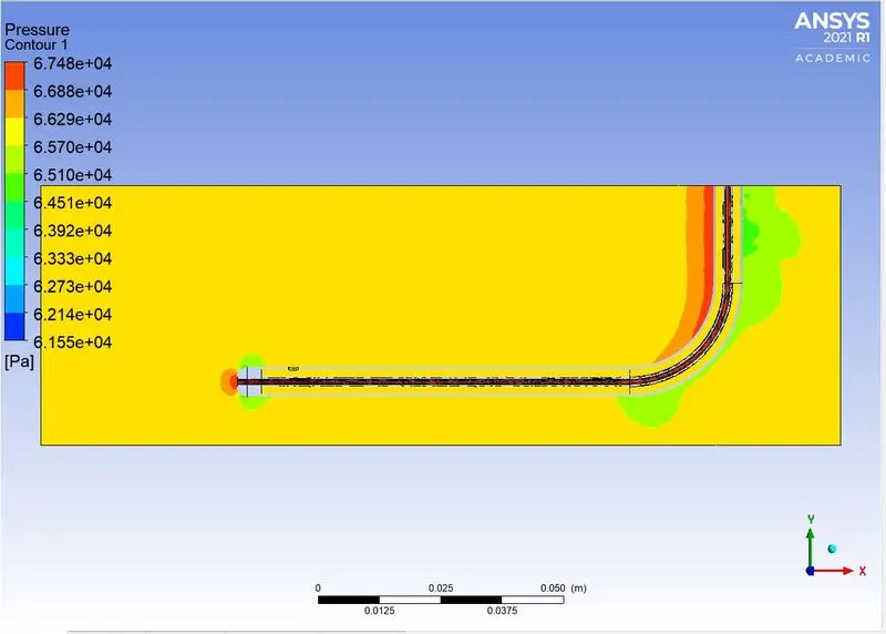
Now from the surface integral option, we obtain the total and static pressure as
`P_t = 67447.029 Pa`
`P_s= 65733.491 Pa`
Substituting the values into the velocity equation derived earlier
`U = sqrt{frac[2xx(67447.029-65733.491)]0.86`
`U = 63.12 m/s`
PITOT TUBE SIMULATION [v = 100m/s]
For the simulation part, we are going to import the mesh file directly into the Fluent solver as shown below
The pitot tube is shown in the fluent solver which will be placed within a enclosure for the flow to take place from inlet of pitot tube towards the outlet to measure the velocity of the fluid stream.
The above image shows the enclosure clearly with holes on the top to measure the static and dynamic pressure.
Setup
The simulation was setup as follows
- Solver - Pressure solver
- Solver Type - Steady
- Viscous - Laminar Flow
- Density = 0.86 `[kg]/m^3`
- Boundary Conditions
Inlet
- Inlet - velocity inlet
- Velocity = 100 m/s
- Pressure = 33287 Pa
Outlet
- Outlet - Pressure Outlet
- Pressure = 33287 Pa
Solution
Results
Pressure Contour
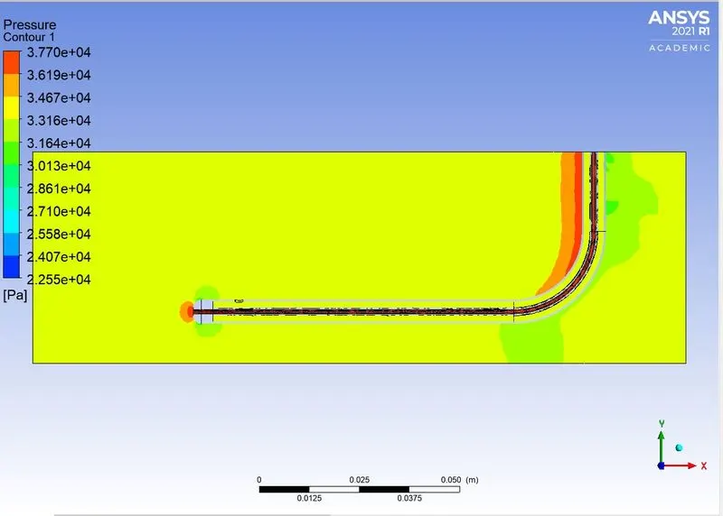
Now from the surface integral option, we obtain the total and static pressure as
`P_t = 37613.417 Pa`
`P_s= 33164.285 Pa`
Substituting the values into the velocity equation derived earlier
`U = sqrt{frac[2xx(37613.417-33164.285)]0.86`
`U = 101.71 m/s`
PITOT TUBE SIMULATION [v = 240m/s]
For the simulation part, we are going to import the mesh file directly into the Fluent solver as shown below
The pitot tube is shown in the fluent solver which will be placed within a enclosure for the flow to take place from inlet of pitot tube towards the outlet to measure the velocity of the fluid stream.
The above image shows the enclosure clearly with holes on the top to measure the static and dynamic pressure.
Setup
The simulation was setup as follows
- Solver - Pressure solver
- Solver Type - Steady
- Viscous - Laminar Flow
- Density = 0.86 `[kg]/m^3`
- Boundary Conditions
Inlet
- Inlet - velocity inlet
- Velocity = 240 m/s
- Pressure = -2817 Pa
Outlet
- Outlet - Pressure Outlet
- Pressure = -2817 Pa
Solution
Results
Pressure Contour
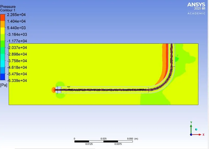
Now from the surface integral option, we obtain the total and static pressure as
`P_t = 22062.621 Pa`
`P_s= -3512.386 Pa`
Substituting the values into the velocity equation derived earlier
`U = sqrt{frac[2xx(22062.621+3512.386)]0.86`
`U = 243.87 m/s`
PERCENTAGE ERROR
| Case | Given Velocity(m/s) | Simulation Velocity (m/s) | Percentage Error |
| 1 | 62 | 63.12 | 1.8064 |
| 2 | 100 | 101.71 | 1.71 |
| 3 | 242 | 243.87 | 0.7727 |
CONCLUSION
- The velocity was measured with the help of total and static pressure
- The percentage of error is very marginal compared to the given boundary condition of velocity
- The simulation was completed and the results are quite accurate.
- A literature review on the pitot tube was done.