Week 3: Flow over a backward facing step
AIM: The main objectives of the current study are as follows:-
1) To setup the case in CONVERGE and simulate the flow over a backward-facing step.
2) To get the pressure & velocity contours as well as plots for pressure, velocity, mass flow rate, and total cell count.
3) Run the simulation for 3 different mesh sizes and compare the results.
4) To find out flow separation characteristics.
INTRODUCTION:
Fully developed flow enters the domain, when the flow reaches the step, because of the expansion of the flow channel, pressure gradient exists, it detaches and a recirculation zone is formed. A turbulent boundary layer encounters a sudden back step, causing flow separation. Later the flow eventually reattaches to the bottom wall as shown in the figure below.
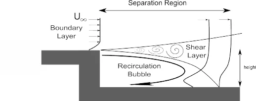
Flow over a backward-facing step (BFS) is a common phenomenon in engineering applications, such as the internal flows in diffusers, turbines, combustors, or pipes, and external flows over aircraft, around buildings, or flows over stepped channels. In these situations, the flow experiences an adverse pressure gradient, which causes the boundary layer to separate from the solid surface. This type of flow is one representative model for flow separation caused by the sudden expansion of the flow domain. It is a basic model that involves the most important features of a separated flow: free shear flow separation, vortex evolution, and re-attachment. The presence of a separated flow, together with a reattaching flow, gives rise to increased unsteadiness, pressure fluctuations, structure vibrations, and noise. The figures given below gives a brief idea about how the flow separation takes place in flow over a backward-facing step and the important regions in the separated flow.
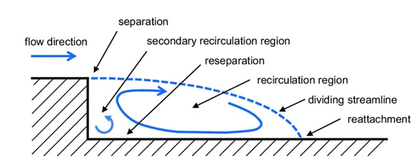
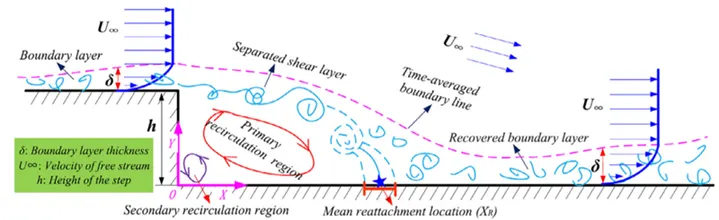
Turbulent flow over a backward-facing step is one of the classical tests to validate turbulence models in CFD. In the present work, steady-state turbulent flow over a backward-facing step was simulated using Converge with the Renormalization-group (RNG) k-ε model to account for turbulent viscosity.
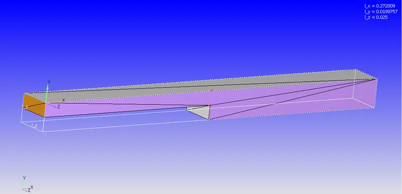
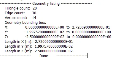
Geometry creation:- The geometry for flow over a backward-facing step is created in CONVERGE by using different commands provided in the create geometry box. The created geometry and its dimensions are shown below:
Case setup for Simulation:
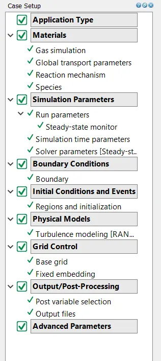
This is the case setup tree that is available in CONVERGE where we select and input all the parameters that are necessary for our simulation.
- Application Type – Time-Based
- The flow is a general gas flow that contains the air as a Material.
- Air contains a Species mixture of O2 and N2 which will flow through the created geometry.
- Global Transport Parameters the Prandtl number is 0.9 and the Schmidt number is 0.78.
Simulation Parameters:
- In the Run Parameter: Steady-state solver is used and the simulation mode is Full hydrodynamic & in the misc. option we enable the Solve Momentum, Solve Species, and Steady-state Monitor.
- In the Steady State Monitor, the minimum number of cycles to be executed for steady-state solver are chosen to be 5000 and the sample size is 100 cycles. This means that the values will be monitored for every 100 cycles after completing 5000 cycles.
- In Simulation time Parameters we set the values for start time as 0 cycles and end time 15000 cycles, the initial and Minimum time setup for 1e-6, max. convection CFL limit to 1 & the remaining values is set to default.
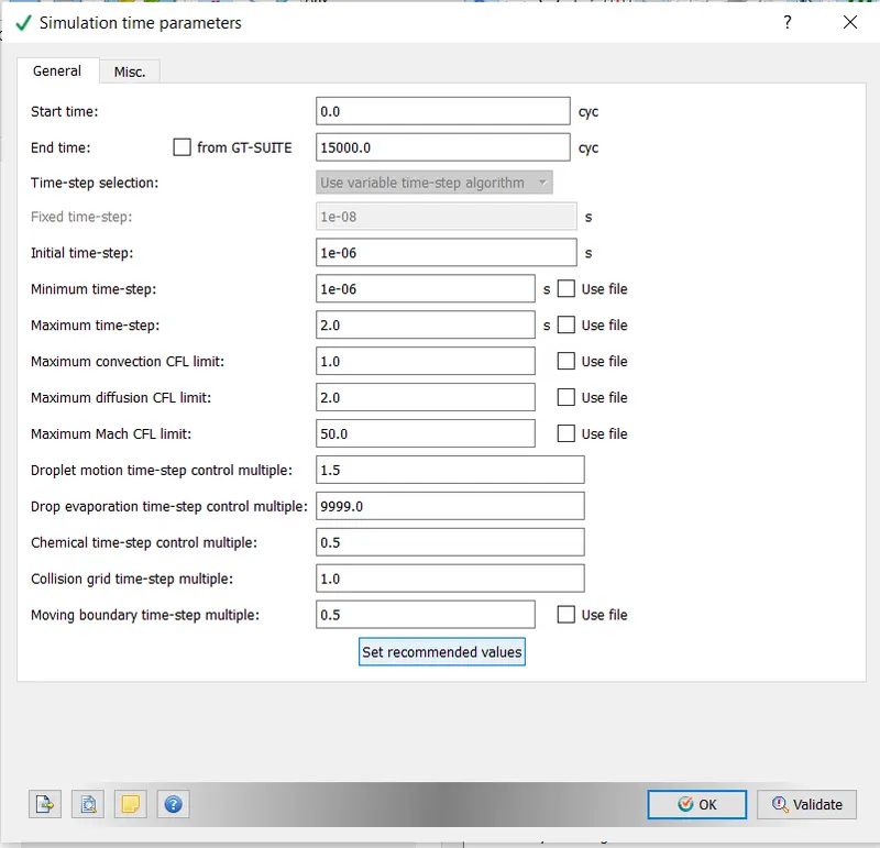
- In the Solver Parameters, the Navier stock equation should be Pressure based solver and the maximum convection CFL limit at the final stage should be set to less than 1.0 & the remaining should be set to default.
Boundary Conditions:
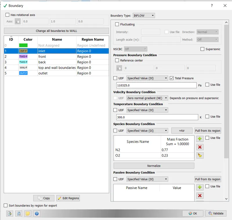
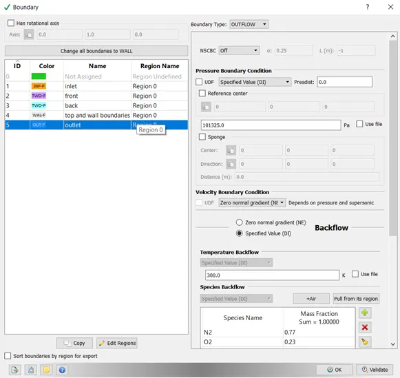
- The boundary conditions for the inlet and outlet are shown in the figure above.
- For front and back we chose 2D boundaries i.e. we are neglecting the length in the Z direction.
- The top and wall boundaries are the wall type with a Law of wall boundary condition and temperature 300k.
Physical Models:
- In the physical models, the Turbulence Modelling is enabled and the solver is selected as RNG K-e and the remaining values are set to default.
Grid Control:
- In the Grid control enable the Fixed Embedding and Base grid.
- In the base grid option, we put the base grid size values in dx, dy, dz directions for different cases.
For this project we are using,
Mesh size For case-I: dx=dy=dz=2e-3m
Mesh size for case-II: dx=dy=dz=1.5e-3m
Mesh size for case-III: dx=dy=dz=1e-3m
In fixed embedding, the following conditions were chosen,
- Entity type=Boundary
- Boundary ID=top and wall boundaries
- Mode =Permanent
- Scale=1
- Embedded layers=1
Output and Post Processing:
- Post variable Selection and Output files are the default values.
- In the output files, we have given a time interval to write the 3D output data file =100 cycles, thus the outputs of the simulation files will be stored after 100 cycles and a maximum of 3 restart files will be saved.
Post-Processing:
I have done the post-processing of the results for all three cases using the CONVERGE STUDIO and ParaView. Post-processing is done to get desired results i.e. various plots and contours for different quantities after running the simulation.
Results and discussion:
1. Mesh generation
a. case 1)
For case 1, the base mesh grid size chosen is 2e-3m, and the results obtained in ParaView are shown in the figure below:
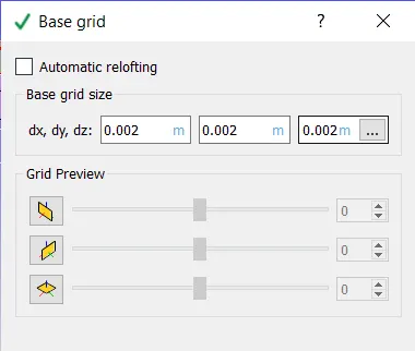
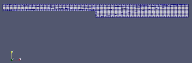
The no. of cells generated in case 1 are 7417 and the no. of points are 28633.
b. case 2)
For case 2, the base mesh grid size chosen is 1.5e-3m, and the results obtained in ParaView are shown in the figure below:
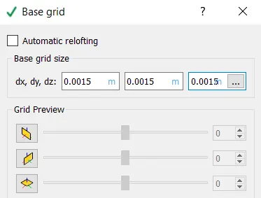
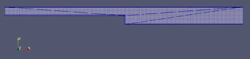
The no. of cells generated in case 2 are 11412 and the no. of points are 43040.
c. case 3)
For case 2, the base mesh grid size chosen is 1.5e-3m, and the results obtained in ParaView are shown in the figure below:
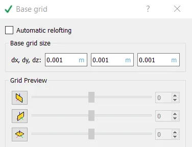
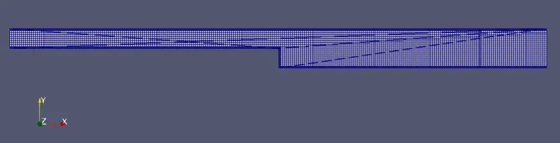
The no. of cells generated in case 3 are 20771 and the no. of points are 76779.
2. Velocity Contours:
CASE I:
CASE II:
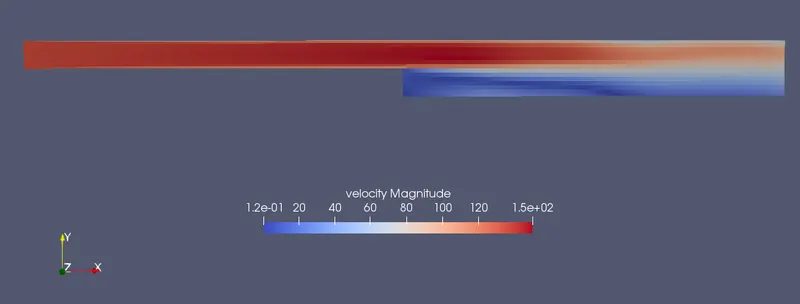
CASE III:
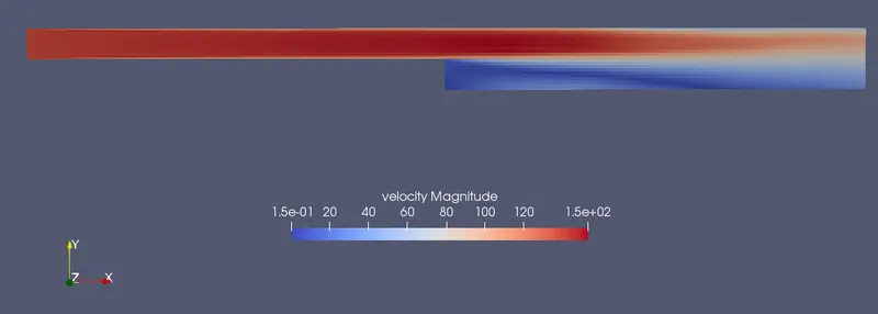
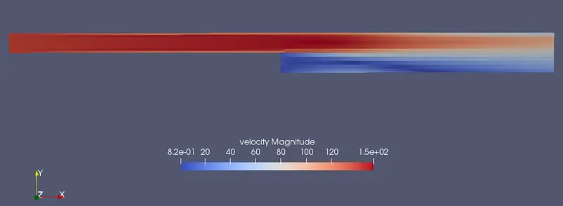
The velocity contours representing the flow over a backward-facing step are shown in the figure above. The velocity is highest at the inlet with a 150 m/sec and at the outlet, the velocity gradually declines approximately to 80 m/sec due to an increase in the flow area and the velocity near the step is very low due to the sudden increase in the area and the flow is turbulent so the pressure drop takes places and thus, the velocity starts decreasing from this point only.
And if we look at the images closely, the image from case 3 gives more clear idea about the exact location of velocity fluctuations from inlet to outlet. Though the difference is not looking much, it can be concluded that with finer mesh size we get more precise results.
Velocity animation:
Pressure Contours:
CASE I:
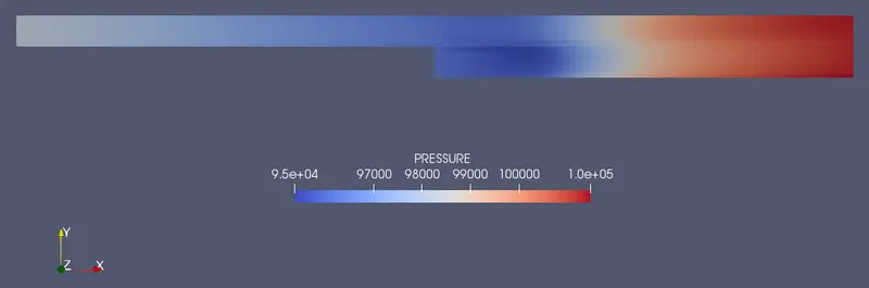
CASE II:
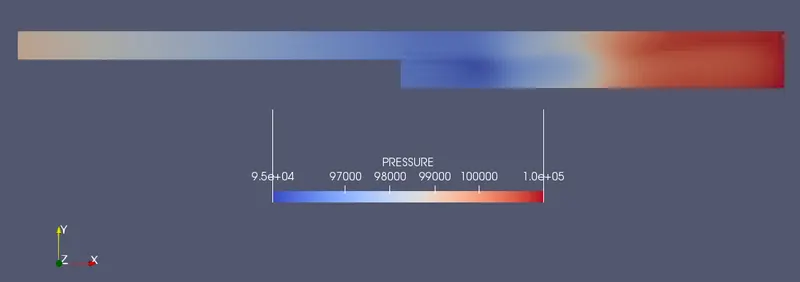
CASE III:
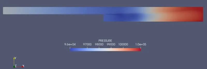
Initially, the pressure is high at the inlet and it goes on increasing until it reaches the step region and after that, the pressure gradually decreases in the step region due to the turbulence caused by sudden expansion, the flow experiences an adverse pressure gradient, which causes the boundary layer to separate from the solid surfaces and after that, there is tremendous growth in the pressure until it reaches the outlet and attains the maximum pressure.'
Pressure Animation:
Pressure plots:
Case 1:
Case 2:
Case 3:
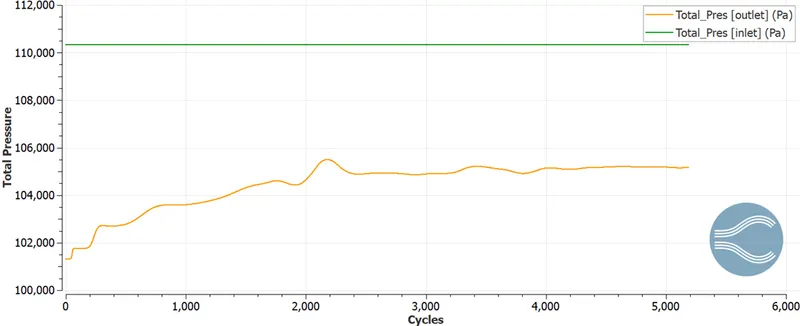
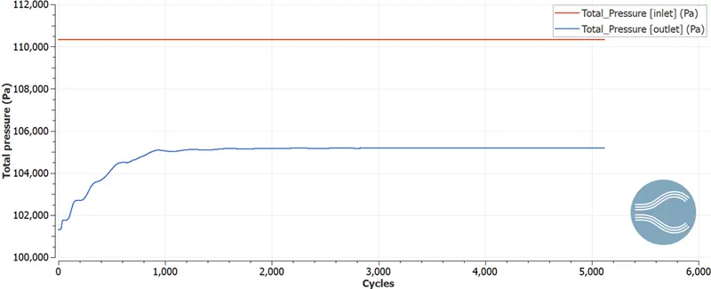
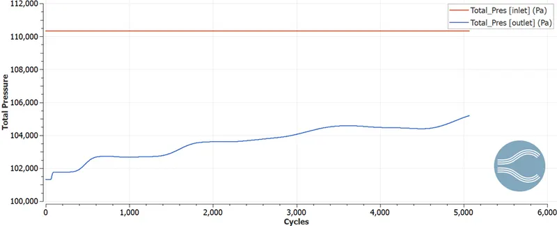
The total pressure is constant at the inlet and the pressure at the outlet gradually increases till it reaches convergence. To get a better comparative idea between the 3 cases below is the plot that combines the total pressure curve for all 3 cases.
COMBINED PLOTS:
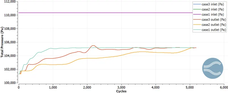
The simulation ran for 5000 cycles in all the cases. In case 1, the total pressure curve converged at about 1500 cycles. whereas for cases 2 & 3 precise cycle number for convergence can not be decided from the above graph as the curves seem to be fluctuating even after 5000cycles are completed. But the simulation stopped because the fluctuations after 5099 cycles must have been in the permissible range.
Velocity plots:
Case 1:
Case 2:
Case 3:
COMBINED PLOTS:
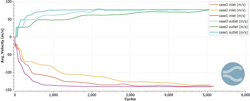
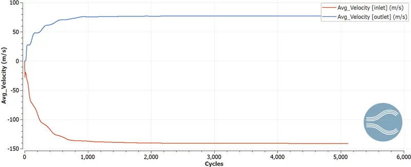
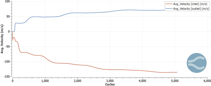
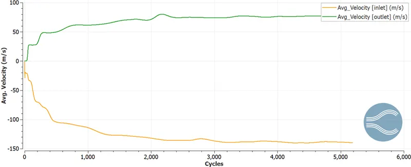
The Velocity at the inlet is about -140 m/sec and the velocity at the outlet about 70 m/sec. The velocity is high at the inlet and low at the outlet because of the increased cross-sectional area at the outlet when compared with the cross-sectional area of the inlet. The velocity at the outlet is almost halved as compared to inlet velocity because the cross-sectional area is doubled. This accounts for the conservation of momentum as there is no entrance or exit of mass between inlet and outlet thus, change in velocity is proportional to change in the cross-sectional area.
Mass flow rate plots:
Case 1:
Case 2:
Case 3:
COMBINED PLOTS:
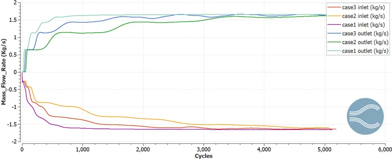
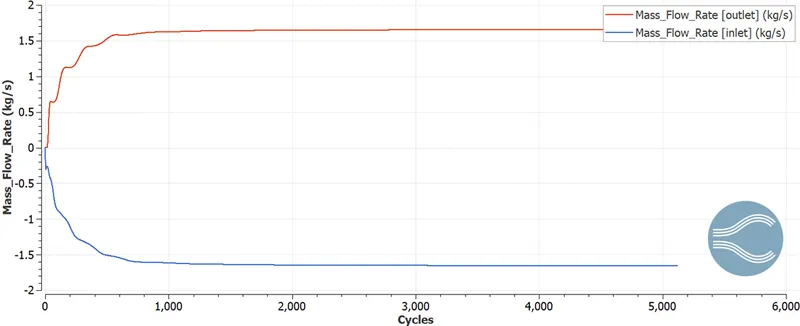
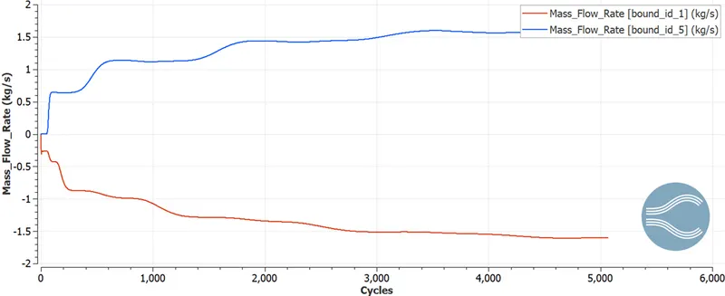
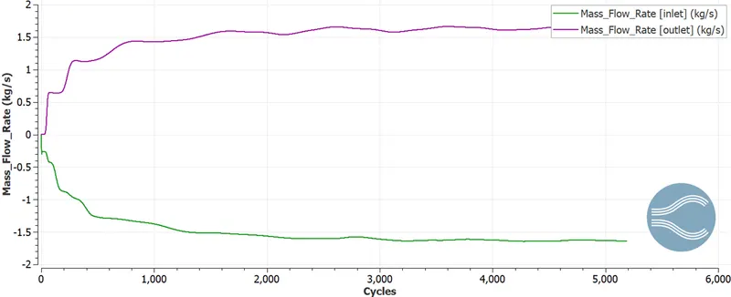
The mass flow rate is the same for both inlet and outlet they are like mirror images. The value of mass flow rate is about 1.7 kg/sec and is converged at different cycle numbers for the 3 cases. The least number of cycles are required for case 1 while max cycles are required for case 3 for the solution to get converged. Thus it can be concluded that finer mesh size requires more number of cycles i.e. requires more computational resources than a coarse grid but the results obtained are also more precise.
Total cell count:
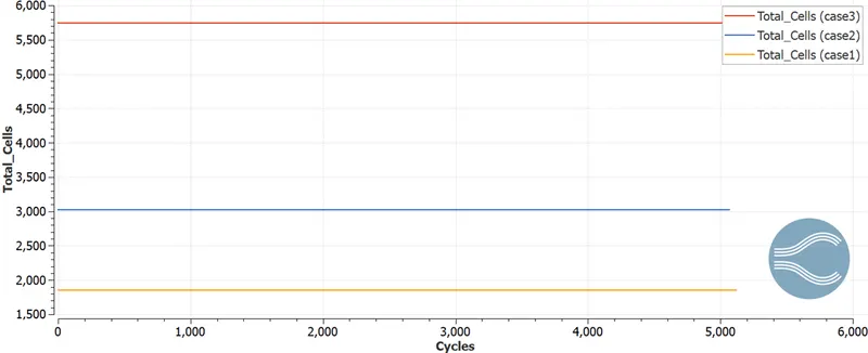
The total number of cells is 5742 for case 3, 3021 for case 2, and 1851 for case 1. The number of cells is increased because of the more refinement of mesh and the outputs of all graphs and plots are smooth and fine as the number of cells is increased.
CONCLUSIONS:
1] The simulation was run for 3 different mesh sizes.
2] Flow variables were plotted against the number of cycles.
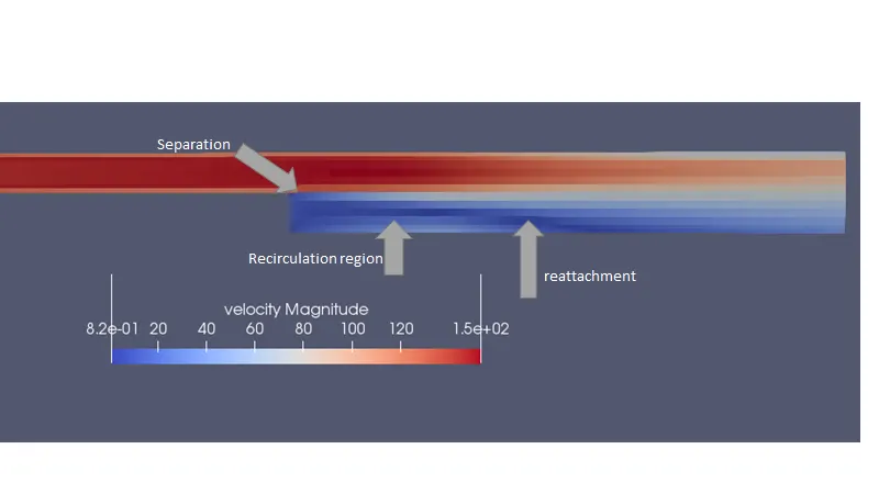
3] Above figure shows all the 3 important zones i.e. the separation zone, recirculation zone, and the reattachment zone.
4] The simulation ran for almost 5100 cycles. More number of iterations are required if the mesh size is finer and I find that case 3 results are the most appropriate as it is the finest mesh size. 6000 to 7000 iterations are enough for obtaining the same average result for all three cases.