Week 3: Flow over a backward facing step

1. Title – Flow over a backward facing step.

2. Objective –

• To create the model of backward step in converge Software.
• To set up the case with proper grid size, material and boundary conditions.
• To solve the case using Cygwin terminal and convert the result for Paraview software.
• To import output files in Paraview and generate required contours and plots.

3. Introduction –

Backward-Facing Step flow is one representative model for separation flows, which can be widely seen in aerodynamic flows engine flows, condensers, vehicles, heat transfer systems, and even the flow around buildings, etc. The flow separation after a simple stage will introduce separation bubble formation, evolution and re-attachment process, which is dependent on the backward facing step geometric design, the inlet and outlet conditions, turbulent intensity, as well as heat transfer conditions. In this study we are simulating flow over a backward facing step to see wake region of flow.

Flow separation – When fluid flows around sloid bodies, then it tries to follow the profile of solid surface. In the case of sharp transitions or when flowing around blunt bodies, the fluid is often no longer able to follow the profile. The boundary layer or flow begins to detach itself from the body surface. This is referred to as a boundary layer separation or flow separation. Downstream of the separation point, vortices often form, resulting in a turbulent flow.

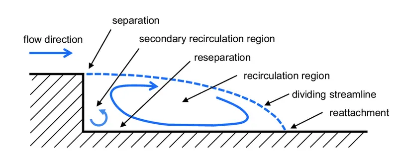
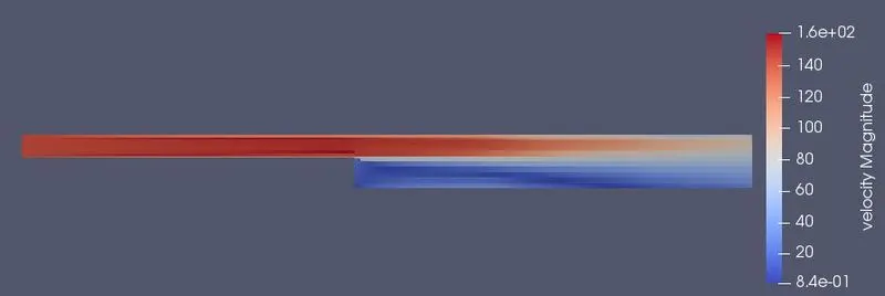
Recirculation region is the region where low pressure due flow separation suck fluid back from main stream. In our simulation sudden expansion of area leads to flow separation, in backward facing step.

4. Procedure –

Flow over a backwards facing step is a classic CFD test problem which is used extensively for validation of simulation codes. The test problem essentially consists of studying how a fully developed flow profile reacts to a sudden expansion in a channel. The expansion will cause a break in the flow and a recirculation or separation zone will form. The stationary incompressible Navier-Stoke equation are applied to solve the model. The following procedure was followed to simulate flow over a backward facing step –

Geometry -

Backward facing step -

Backward facing step with dimensions-

Case setup -

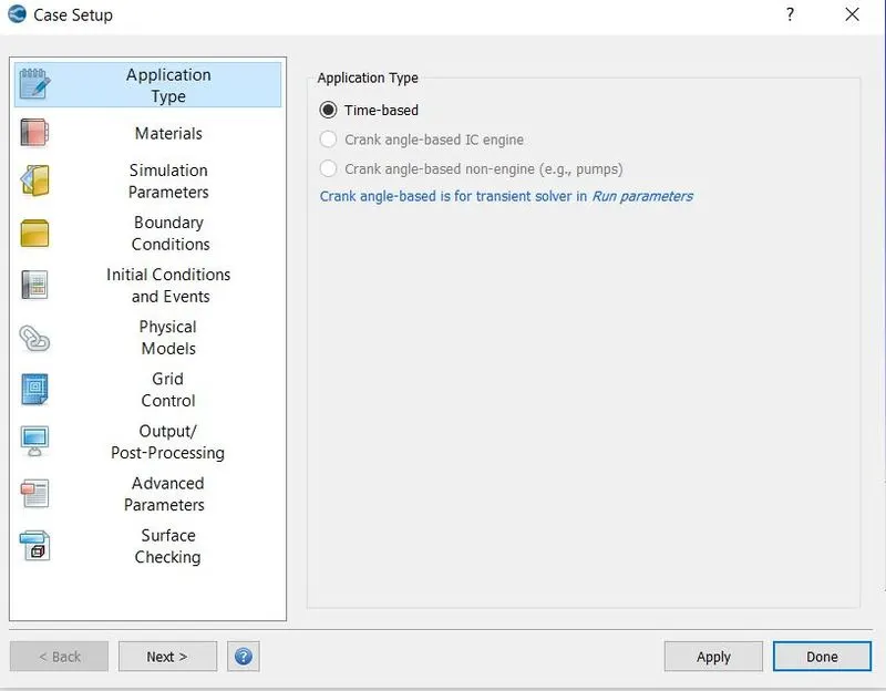
1. Start with the choosing application type, we chose time based this simulating does not related to IC engine or other mechanism with has crack angle parameter.

Case Setup - Application Type -

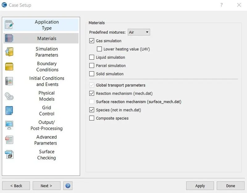
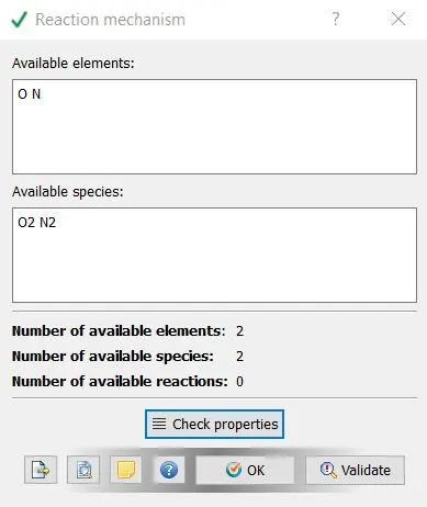
2. Air was chosen as fluid with enabled reaction mechanism.

Material selection -

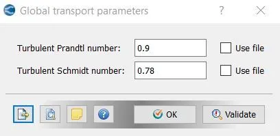
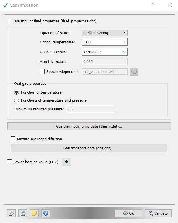
3. Parameters of gas simulation, global transport parameters were kept same.

Global transport parameters -

Reaction mechanism parameter -

Gas simulation parameter -

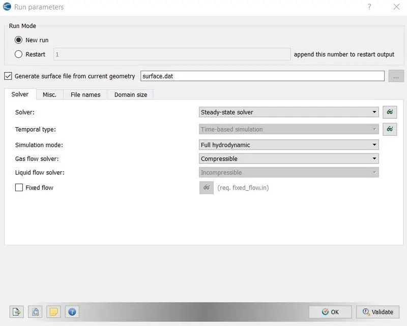
4. In run parameters steady state solver was chosen, because in this simulation fluid is continuous and it gets steady state after some time. Simulation mode is chosen as Full hydrodynamic, because we want to simulate with affect of fluid also, if someone want to see quality of mesh and its effect only, he can go with no hydrodynamic option. Air is compressible so we went with that option.

Run parameters -

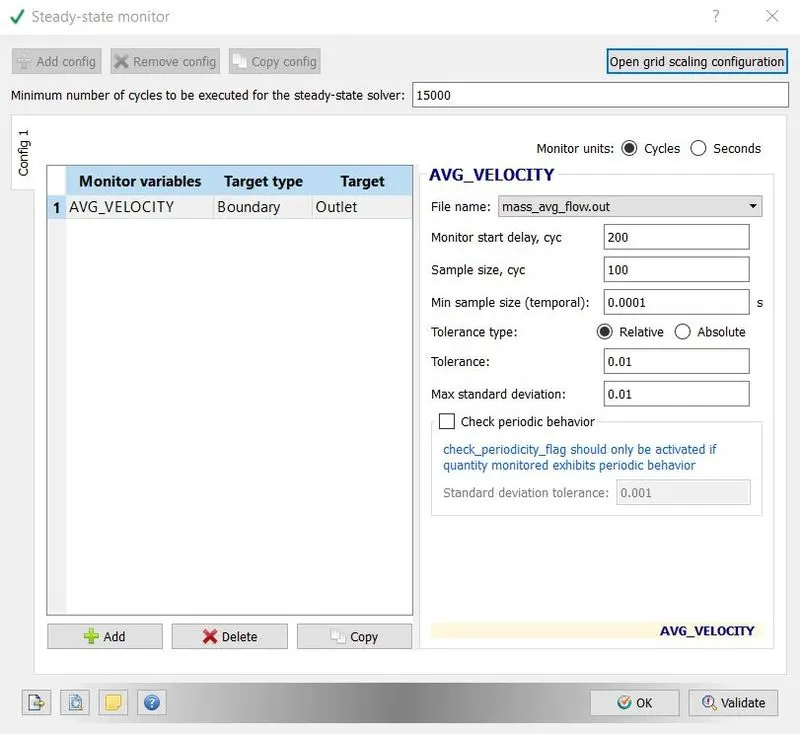
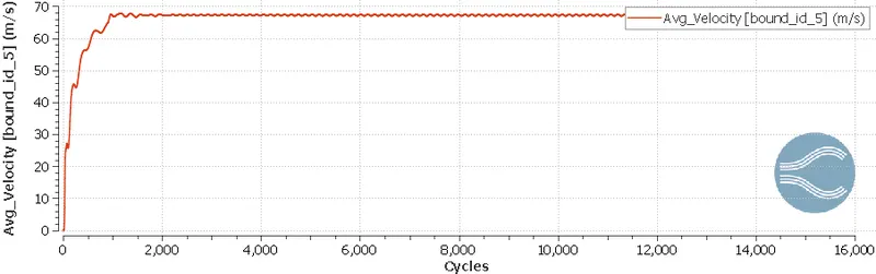
5. If someone want to monitor parameters, he can enable option steady state, we selected average velocity as parameter.

Steady state monitor window -

6. Simulation time parameter is important parameter which decides simulation stability, number of time steps which is iterations, minimum and maximum time step etc. we went with 15000 time steps with stating at 0 second, minimum time step and initial step 1e-06, maximum time step of 1 second. These parameters will affect simulation time. Maximum convection CFL limit was reduced from 10 to 1 to get stable solutions. CFL limit decides the stability of simulation, if it is high than solution will get fluctuations.

Simulation time parameter -

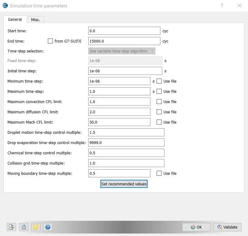
7. In solver parameters pressure based solver was selected and 1 was set as maximum convection CFD limit for final stage.

Solver parameter -

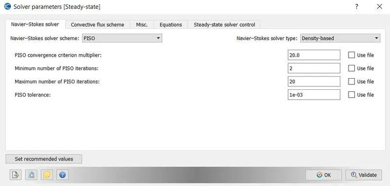
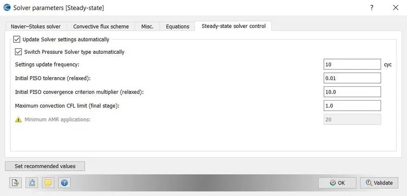
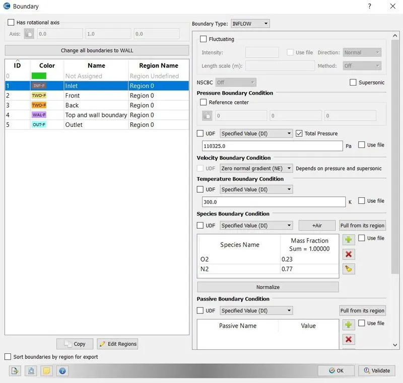
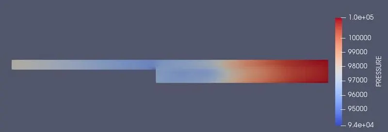
8. In boundary conditions inlet was set with inflow with pressure 110325 pascal and air as fluid. Similarly, at outlet boundary type selected as outflow with pressure 101325 pascal. Front and back walls were kept as 2D because we wanted to convert it into 2D simulation. Top and bottom walls are walls so walls were selected as boundary type.

Boundary conditions -

Inlet -

Outlet -

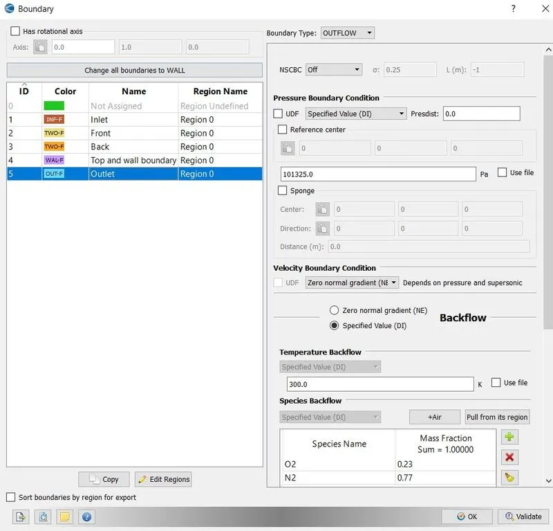
Front and back-

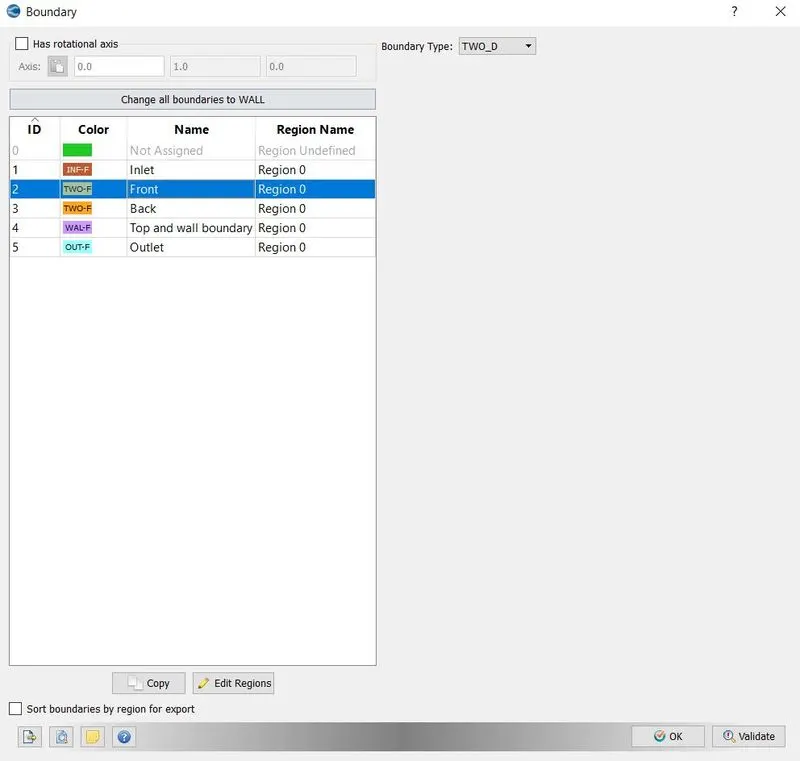
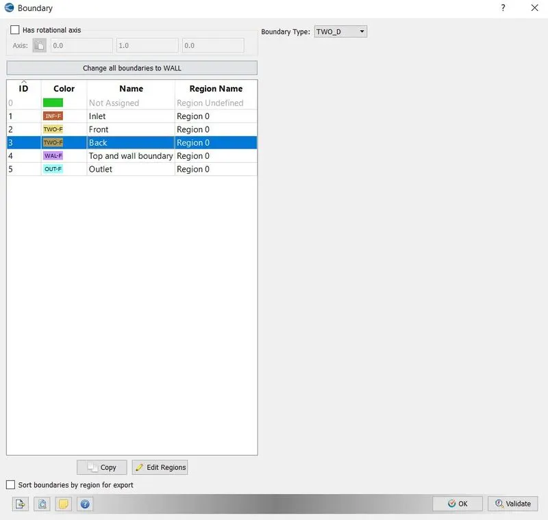
wall -

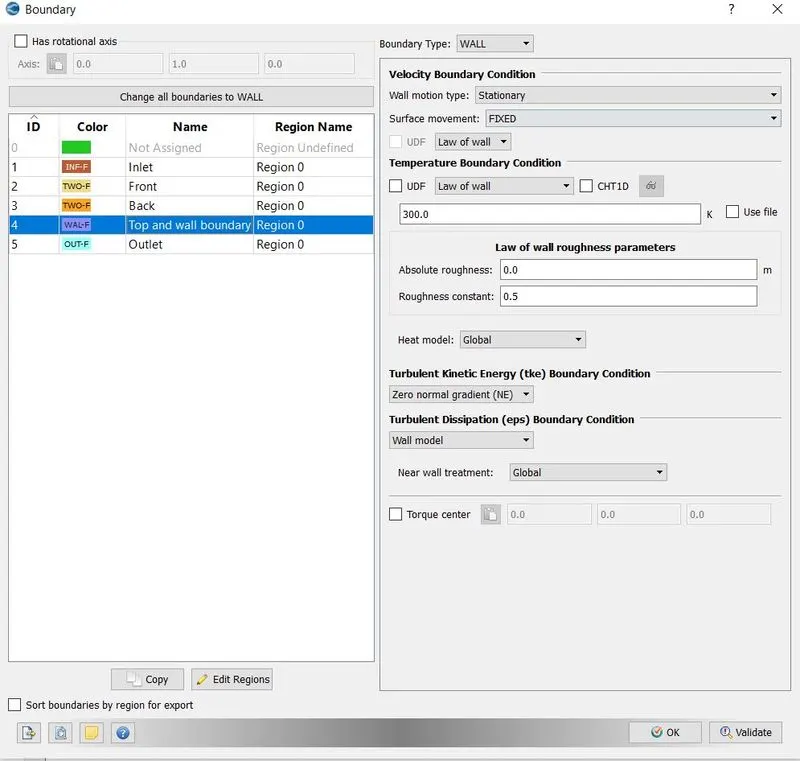
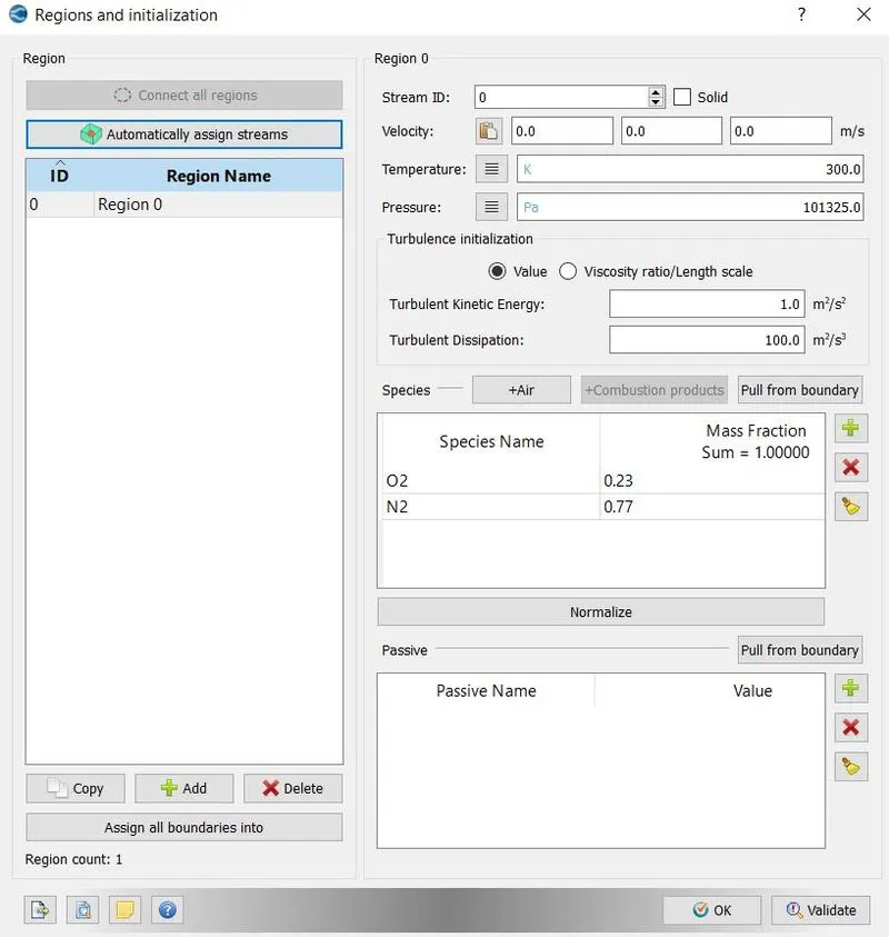
9. Region was created which helps to initialize the solution. In boundary conditions this region was selected for all boundaries as region type.

Regions -

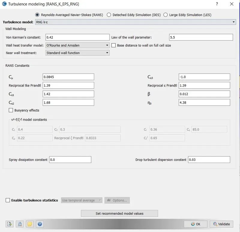
10. Reynolds averaged Navier-Stokes was selected as turbulence model with default parameters.

Turbulence model and its parameters -

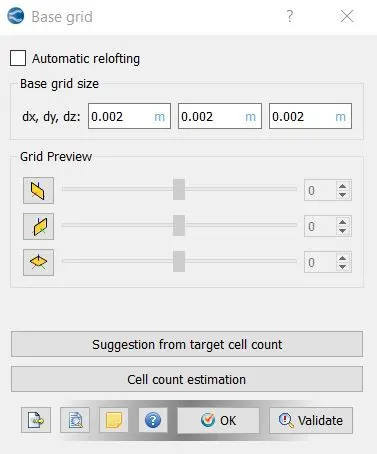
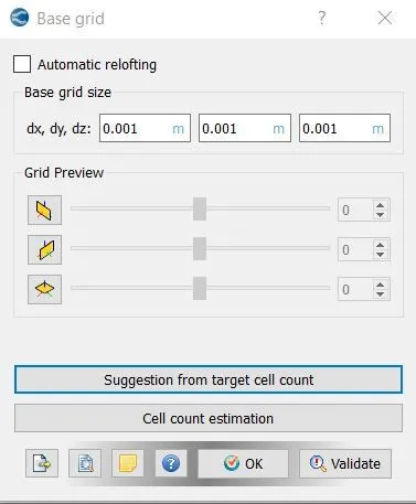
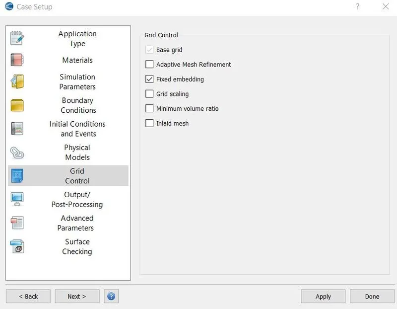
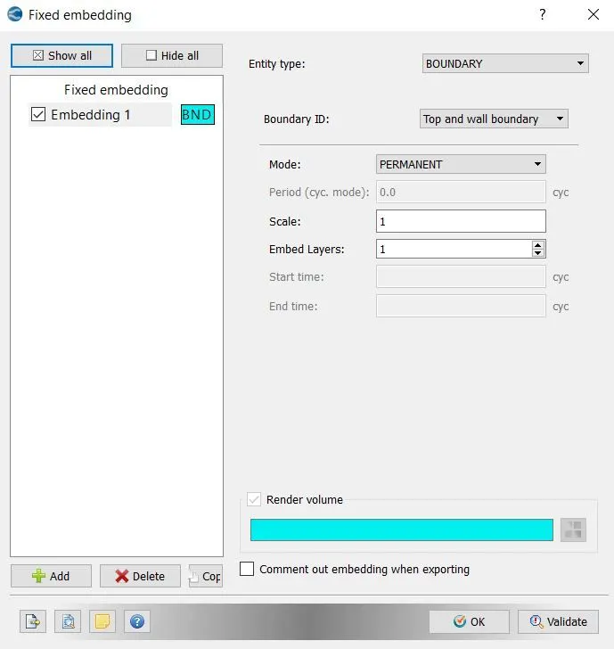
11. In base grid option the size of mesh was selected with option of fixed embedding. This option allows us to refine mesh at particular area like we selected top and bottom wall, where we wanted mesh with the reduced scale of 1 from current size.

Grid size -

Case1 -

Case2 -

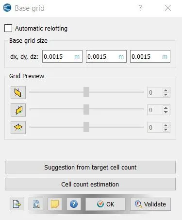
Case3 -

Grid control parameters -

Fixed embedding parameters -

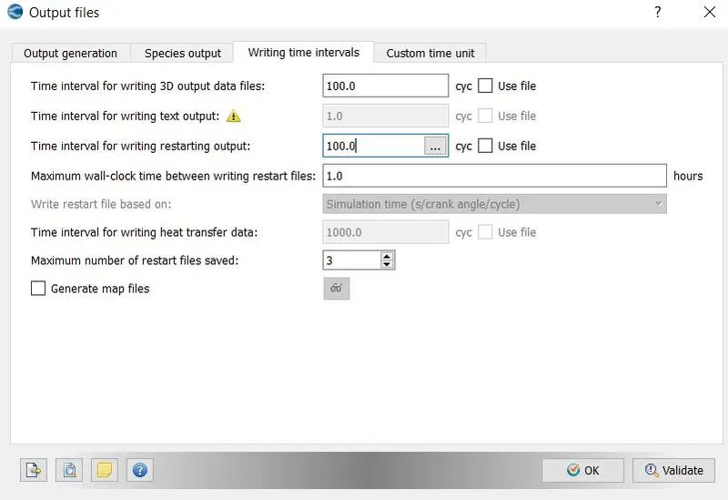
12. Post variable selection was kept unchanged because it has necessary variables selected as defaults. Output files option defines the time interval for writing output data, restarting output etc. we gave 100 as time interval to write data file and time interval for restarting, because we wated 150 output files. We were simulating for 15000 time steps and want a output file after 100 cycle so it is obvious that we will get 150 output files. Restart files allows you to restart simulation from particular time step.

5. Results-

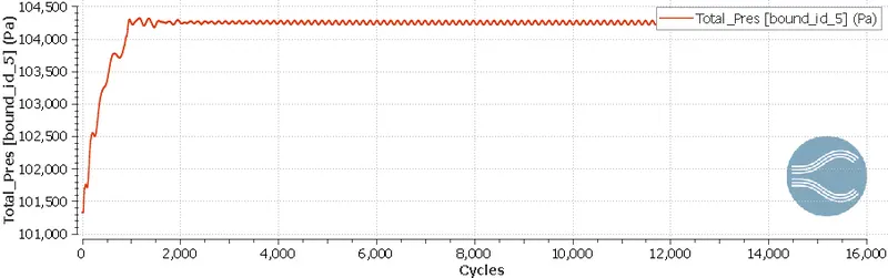
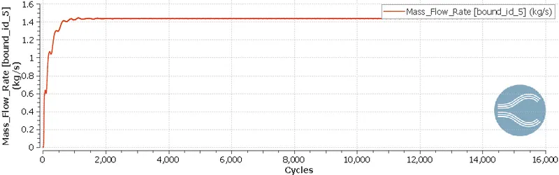
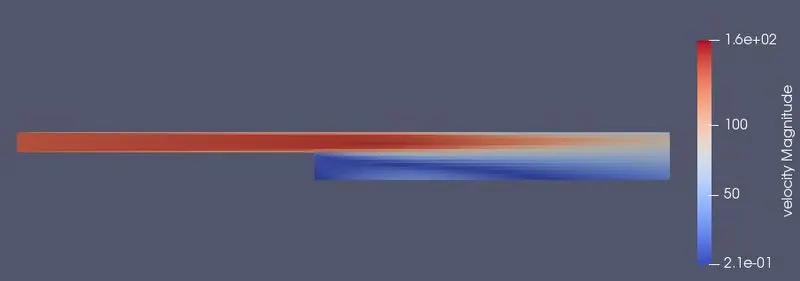
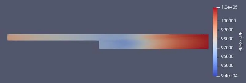
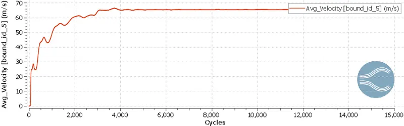
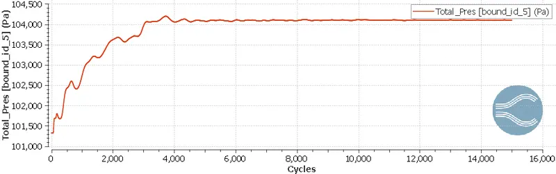
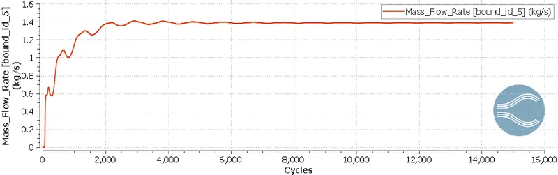
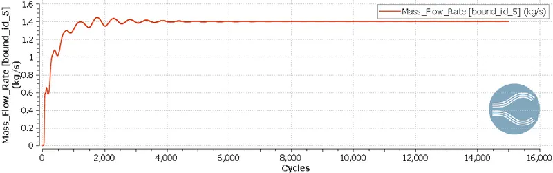
Velocity and pressure contour was created to get clear idea about maximum pressure region and we can visualize area of separation from it also. The pressure difference between inlet and outlet was kept 9000 pascal and it was the only cause of fluid flow. All the parameters get fluctuations at the beginning of simulation and gets steady values after some time.

Case1

Mesh -

Velocity contour –

Pressure contour –

Velocity plot –

Pressure plot-

Mass flow rate –

Cell count –

Case2

Mesh -

Velocity contour –

Pressure contour –

Velocity plot –

Pressure plot-

Mass flow rate –

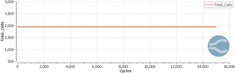
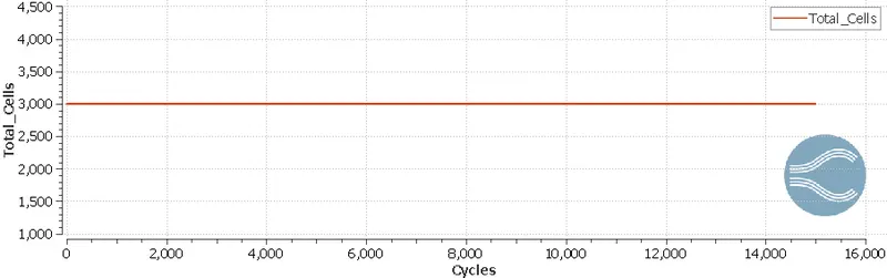
Cell count –

Case3

Mesh -

Velocity contour –

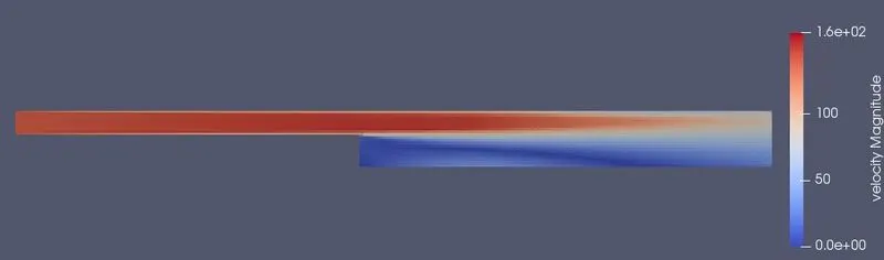
Pressure contour –

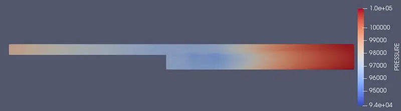
Velocity plot –

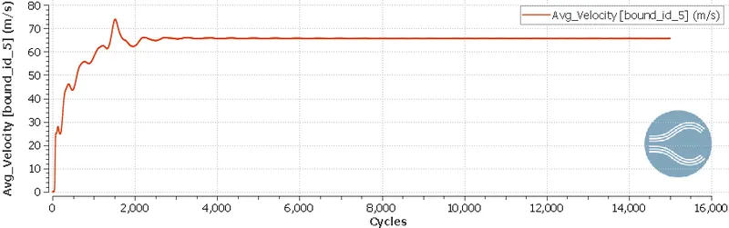
Pressure plot-

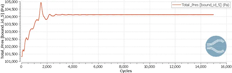
Mass flow rate –

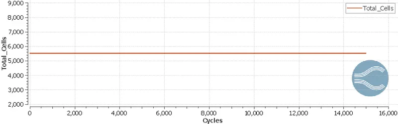
Cell count –

Case/Parameters	Cell count	Average Mass flow rate at Outlet(Kg/s)	Average Velocity at Outlet(m/s)	Average Pressure at Outlet(Pa)
Case1	1943	1.435	67	10450
Case2	2994	1.423	66.2	10420
Case3	5516	1.410	65.7	10412

6. Conclusion –

The experimental study of flow over the backward-facing step was performed. We validated the theory of flow separation and its effect by numerical experiment. Three cases were there, distinguished by grid size only. According to results we can say mesh refinement lead us to perfect results, although it consumes more time. It can be concluded that for all obstructions, the velocities are very small in the recirculation zone compared to the velocity of the mean flow, which results into a strong shear at separation surface.