Week 3: Flow over a backward facing step
Aim : Simulating flow over backward facing step.
Objective :
1. Create a backward facing step geometry in converge.
2. Set a case and simulate for three different base mesh sizes.
Introduction :
Many industrial application involves flow seperation and reattachment, the backward facing step in one where we discuss such phenomenon and the effect due to which flow seperation takes place.
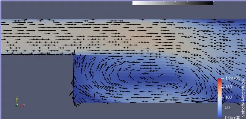
In our simulation the fully developed flow enters the domain from left. When the air or the fluid used reaches the step, because of pressure gradient the expansion in flow occurs which causes it to detach and form a recirculation zone.
Seperation and reattachment of turbulent flow occur in many practical application ex: combusters, diffusers,flow around airfoil and building.
The major reason for flow seperation is adverse pressure gradient which is due to increase in static pressure in flow direction, this causes increase in potential energy and decreases in kinetic energy and showing down a fluid which causes its seperation from wall.
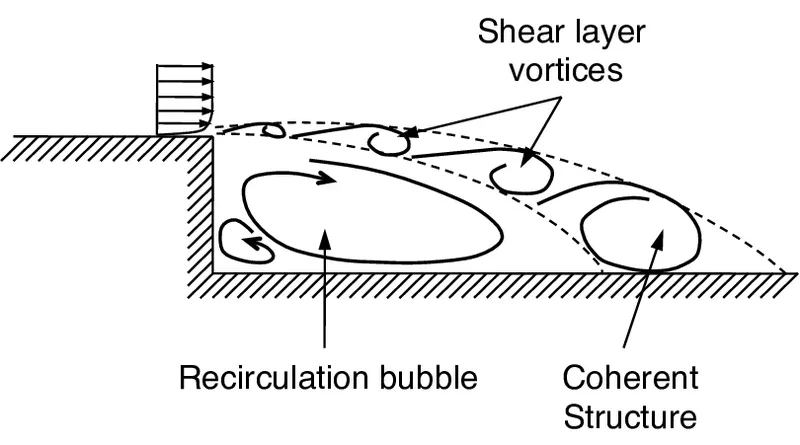
In the above image we can find out all the major regions present in backward facing step flow.
We can create the geometry in Converge CFD software or any modelling software and import it.
Case setup :
1. Mesh sizes
Mesh element sizes in x,y and z-directions.
case 1: 0.001 m
case 2: 0.0007 mm
case 3: 0.0008m
2. Type of simultions : steady -state simulation with zero reactions and only air (77% N2, 23% O2) as the medium of flow.
3. Steady state monitor properties:
a) Average velocity at the outlet
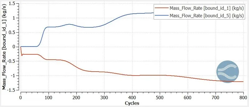
b) Average mass flow rate at the outlet
4. Boundaries :
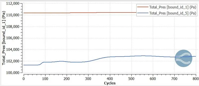
Inlet : Inlet boundary condition with pressure inlet(111325Pa).
Outlet : Outflow boundary condition with pressure outlet (101325Pa)
Top and Bottom : Stationary, no-slip wall.
Front and Back : 2D faces.
Pressure differences between the inlet and outlet = 10000Pa
5. Solver properties :
Deatail : 2 minimum iterations and 20 max iterations per cycle, Tolerance = 0.001
Minimum Cycles = 0
Maximum Cycles = 15000
Minimum time step = 1e-9 sec.
Maximum time step = 1sec.
Maximum convection CFL limit (final stage) = 0.5
6. Turbulence model :
RNG K-epsilon turbulence model
Results :
Case 1: Mesh grid size = 0.001
Mesh :
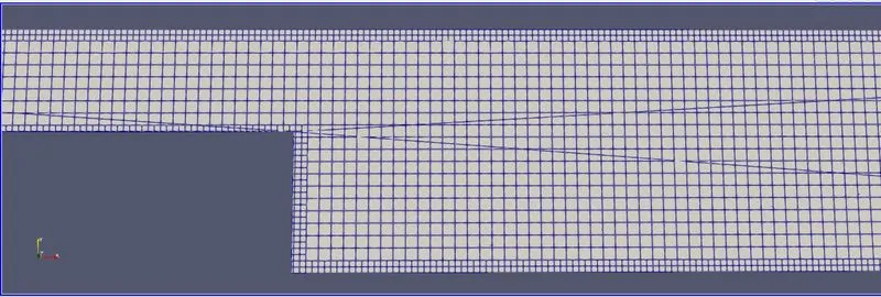
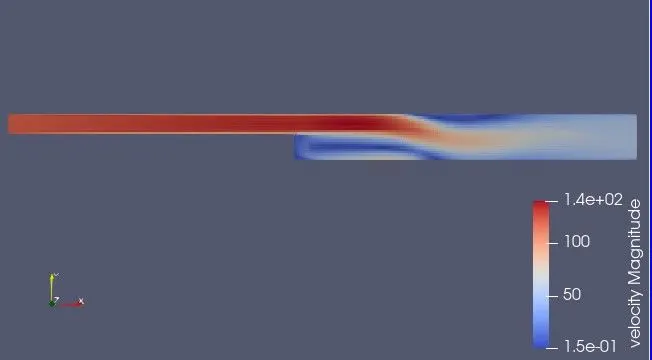
Velocity contour :
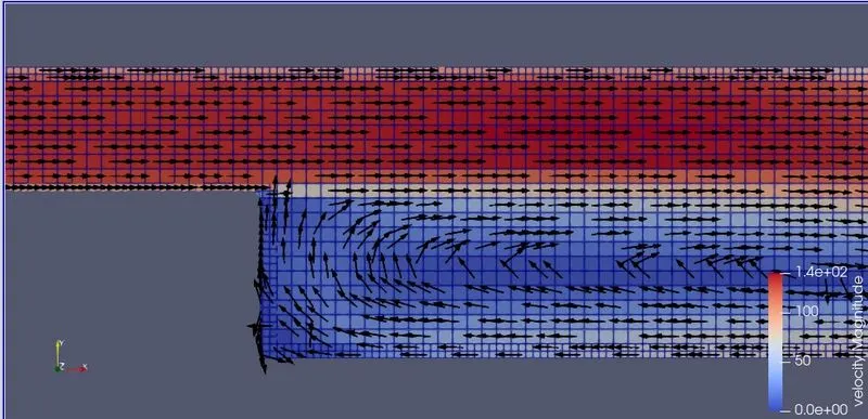
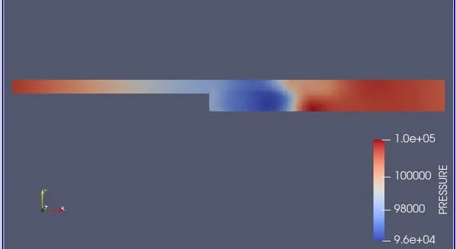
Pressure contour :
Pressure Animation :
Velocity Animation :
Line Plots :
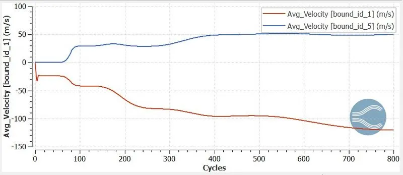
Average Velocity :
Total Pressure :
Mass flow rate :
Cell count :
Case 2: Mesh grid size = 0.0007
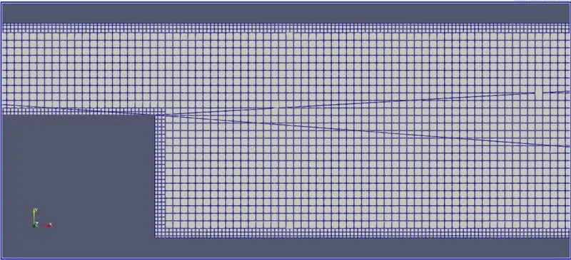
Mesh :
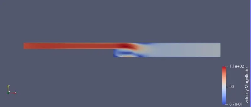
Velocity contour :
Pressure contour :
Pressure Animation :
Velocity Animation :
Line Plots :
Average Velocity :
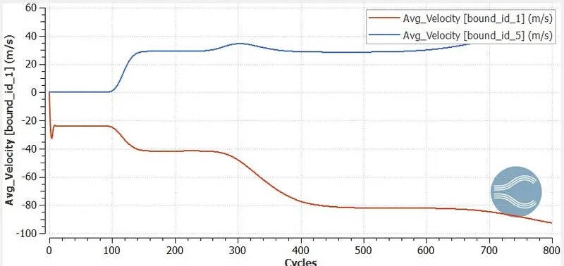
Total Pressure :
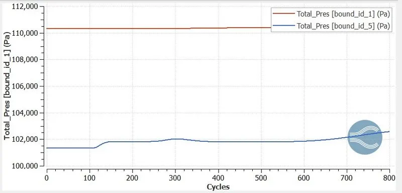
Mass flow rate :
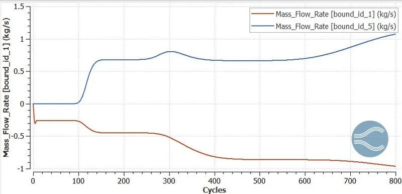
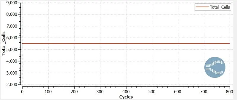
Cell count :
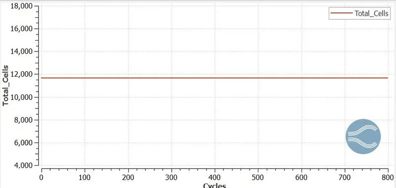
Results :
Case 3: Mesh grid size = 0.0008
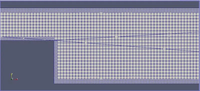
Mesh :
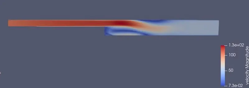
Velocity contour :
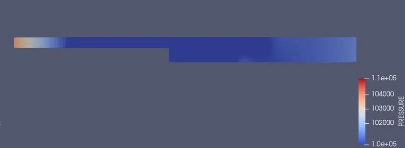
Pressure contour :
Pressure Animation :
Velocity Animation :
Line Plots :
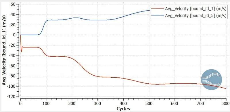
Average Velocity :
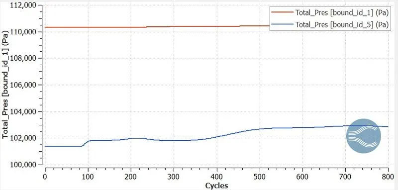
Total Pressure :
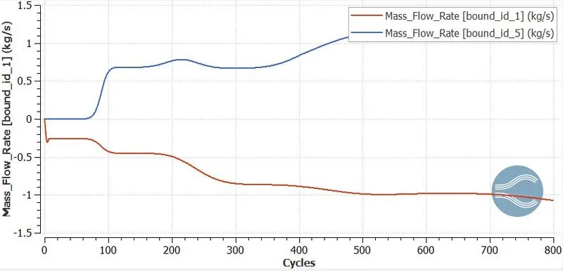
Mass flow rate :
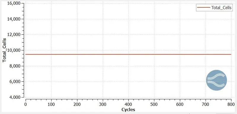
Cell count :
Link of Google drive :
https://drive.google.com/file/d/1gEU7tchNw6d6lR8ZVux-AHwd2PVFtgWA/view?usp=sharing
Conclusion :
The flow simulation of air was performed on the backward-facing step for 3 different mesh sizes and the following conclusion can be shown :
1. The air flows from the inlet to the outlet. The velocity of air is higher at the inlet than at the outlet. This is because of the backward-facing step, which changes the geometry of the fluid domain.
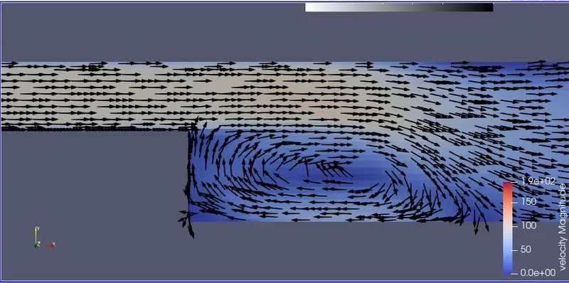
2. Due to the backward-facing step, there is a pressure drop near the step, this causes some fluid particles to flow in the reverse direction, which creates vortices. This can be seen in the vector plot.
3. With the increase in the number of grid elements, the solution obtained becomes more and more accurate. The fluid properties are captured more accurately if the mesh is more refined. This is the reason for the introduction of embedded layers which improves the accuracy of the solution near the walls. In general, the smaller the element size , the more accurate is the solution obtained.
4. With the increase in the number of cells, the solution become more accurate but the computation time increase considerably. Hence, the problem must be studied thoroughly before performing the simulation and it must be decided how much are we willing to compromise the accuracy of the solution to save resources.