Week 3 - External flow simulation over an Ahmed body.

Ahmed body: The Ahmed body was first genetated by S.R. Ahmed. well this is very important benchmark for aerodynamic simulation tools. This a device which had 50-millimeter cylindrical legs attached to the bottom of the body and the rear surface which has a slant that falls of at 35 degrees. It will be clearly shown in the sketch below that it has a length of 1.044 meters, the height of 0.288 meters and the width of 0.389 meters.Please find the following diagram

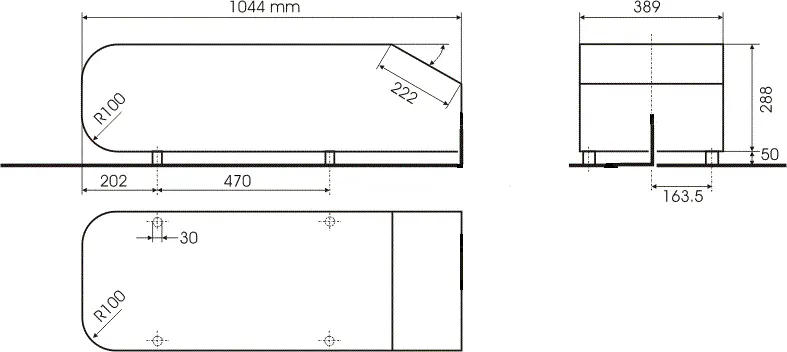
The flow for the model is turbulent which is based on velocity and body length. For the default mesh size in ANSYS-FLUENT we will use k−ε model and for the later stage k−ω SST model is used.

Importance of Ahmed body :

Complex shaped things is very challenging to model and it's difficult to quantify the aerodynamic drag computationally so the Ahmed body is a main model widely used in the automotive industry or Aerospace indutry for validating simulation .

The drag force or moment is an important factor considering fuel consumption. As the drag force increases the fuel consumption also increases which in will effect on structures and cost. As the burning of fossil fuels becomes an issue.

Negative pressure in the wake region

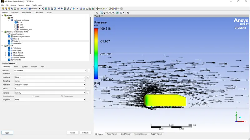
When the air moving over the vehicle or mainly Aeroplanes it makes wake region as there is pressure difference betwwwen the two flowas which is separated at the rear end, it leaves a large low-pressure turbulent region behind the vehicle which is known as the wake. This contributes to the formation of pressure drag which affects the mainly plane performance.

Work flow Approach:

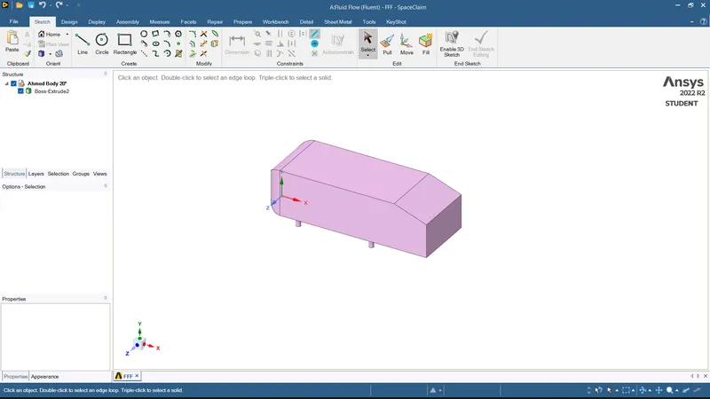
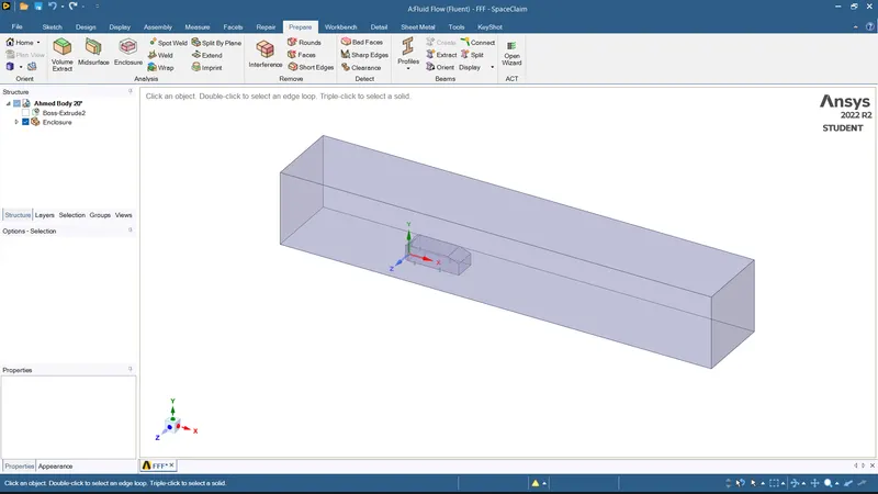
1. Ahmed's body is loaded into the Space claim. And then a single enclosure is drawn throught out Ahmed's body.
2. Then the the geometry is loaded for meshing.
3. A baseline simulation is set up with the default element size of Ansys (413.6 millimeters).
4. A named selection is created for the enclosure viz; inlet, outlet, symmetry.
5. To create the named selection for the car the enclosure faces are hidden, and box select is selected from the meshing toolbar and (car wall) name is given to it.
6. Ansys Fluent window is opened, and the geometry is loaded.
7. Steady-state, the density-based solver is selected.
8. Reference values are updated as per the prescribed conditions.
9. In the inlet boundary condition, inlet velocity is 25 msec and 300 K temperature are set.
10. Drag-coefficient plot and lift-coefficient plot is created by setting the reference as (car walls).
11. Hybrid initialization is selected.
12. The solution is initialized by hitting t=0.
13. The cut-plane-z is created along Ahmed's body.
14. The velocity contour, pressure contour is created along the cut-plane-z.
15. The animation video is created for the velocity contour.
    

Simulation with a finer mesh using k−ω SST.

• when the simulation run successfully. The geometry is loaded into the Space Claim.
• The region of local refinement is created along Ahmed's body.
• As the body is perfectly symmetric, the simulation is executed by considering the only half body. This is the best practice where we can save on the number of cells and get the results faster as well.
• The geometry is loaded for meshing. The multizone method is selected for the outer enclosure to provide hexahedral mesh which provides accurate results in simulation.
• The element size for the first enclosure will vary as (100mm, 90mm, 80mm), the element size for the second enclosure will vary as (50mm, 45mm, 40mm), the element size of the leg of Ahmed's body will be 5mm, the first layer thickness, inflation layer, and the maximum thickness will be varied accordingly to imitate the experimental results.
• The rest procedure is the same as above, the necessary contour plot and graphs have been uploaded respectively.

Preprocessing:

Task1: Creating a external flow simulation over Ahmed body by creating a single closure and using default mesh value of ANSYS-FLUENT

Turbulence model: k−ε

Ahmed body model

Creating an enclosure across Ahmed body

The three planes are normal to the x,y,z axes respectively.

As the body is perfectly symmetric, lets simulate by considering only half the body. we can save the the number of cells here.

To get half of Ahmed's body, the section mode is selected in Space Claim and the front view plain is selected to yield the desired result accordingly.

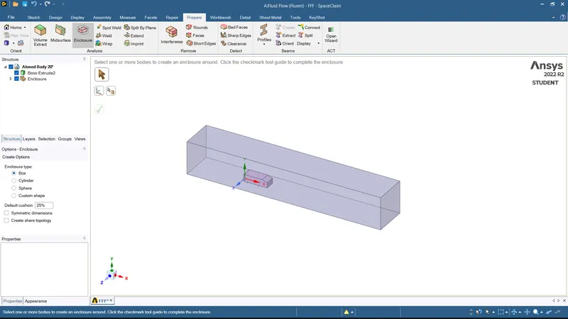
Once the geometry part is complete, it is loaded in the meshing window to perform the baseline meshing.

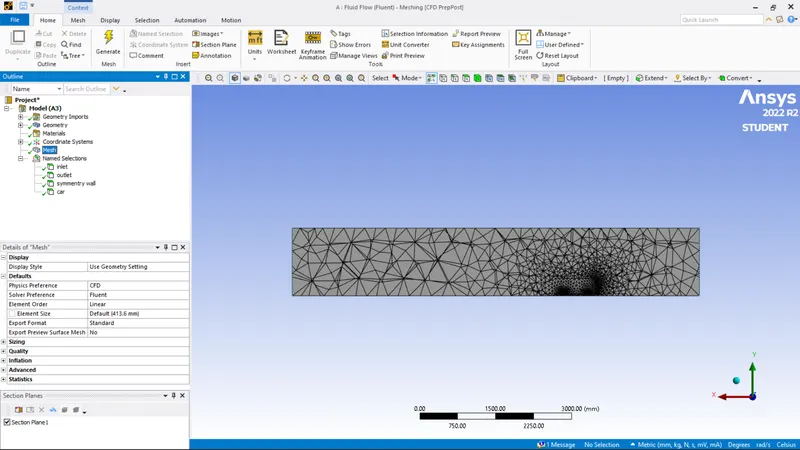
Simulating with a default mesh size of Ansys-Fluent

Creating named selection to set up physics and boundary conditions.

Inlet boundary condition (velocity inlet)

outlet boundary condition (pressure inlet)

Results

Residual plot

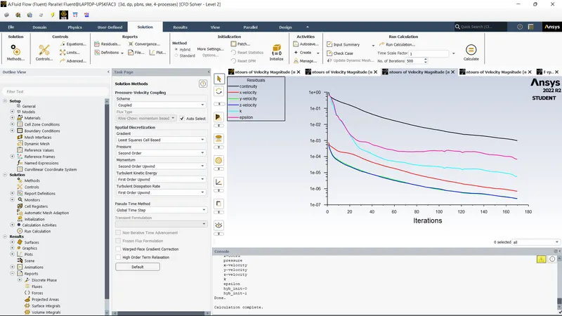
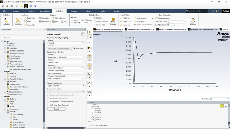
Drag-coefficient plot

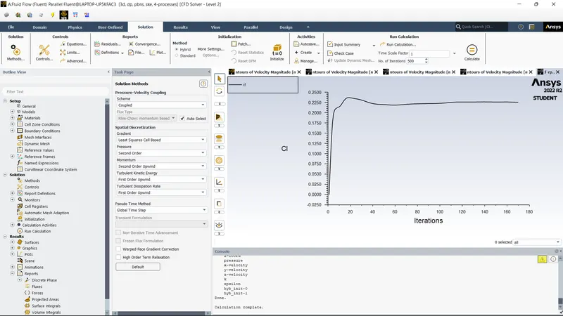
Lift-coefficient plot

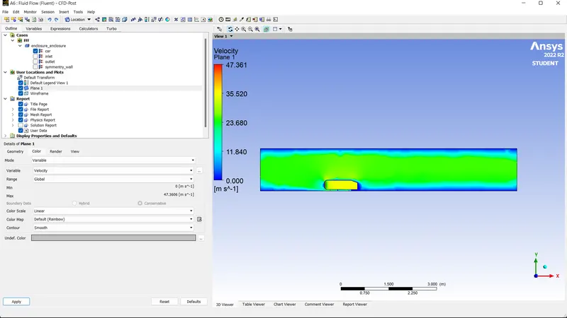
Velocity contour

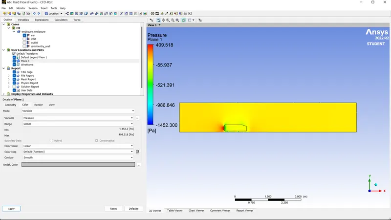
Pressure contour

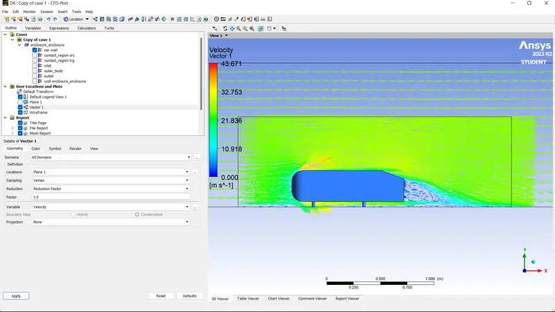
The vector plot showing the wake region

Drag-coefficient is	0.39
Lift-coefficient	0.225

from the following figure that the results of the base simulation are distorted and do not capture the turbulent flow behind the body perfectly. This simulation captures the wake length, high velocity, low-velocity areas which can be used to further refine the mesh value around the Ahmed body and add a local refinement around.

Task2 (a) Creating a External flow simulation over Ahmed body with finer mesh in a double enclosure.

Refinement

A region of local refinement is added to the Ahmed body.

Share Topology: It is set to share. It is used for sharing the information between the two enclosures and to make the mesh uniform.

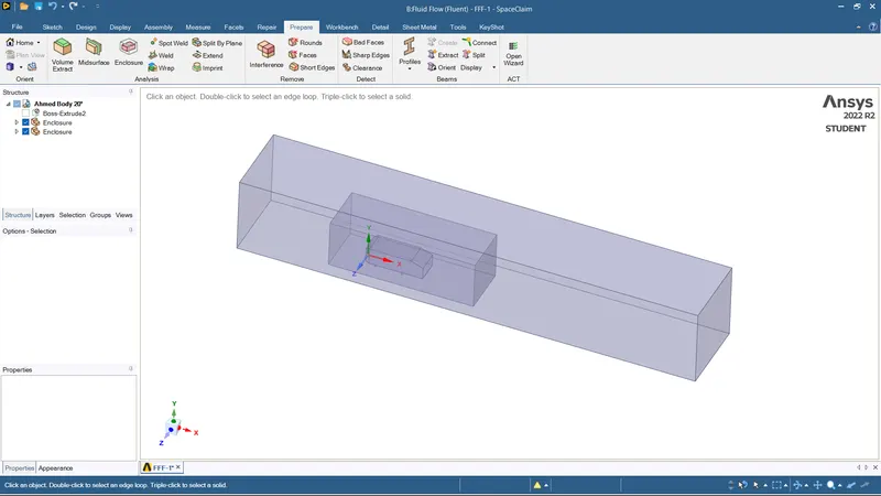
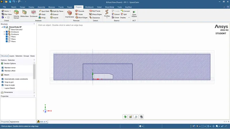
The geometry is loaded into the meshing window.

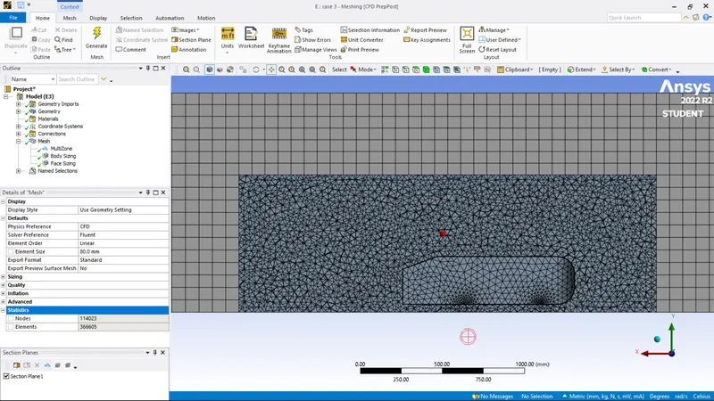
Meshing

The meshing involves the following steps

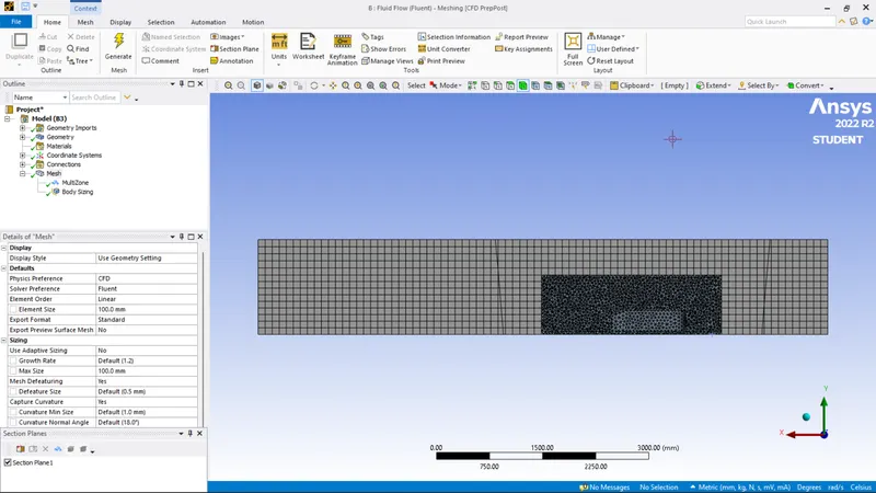
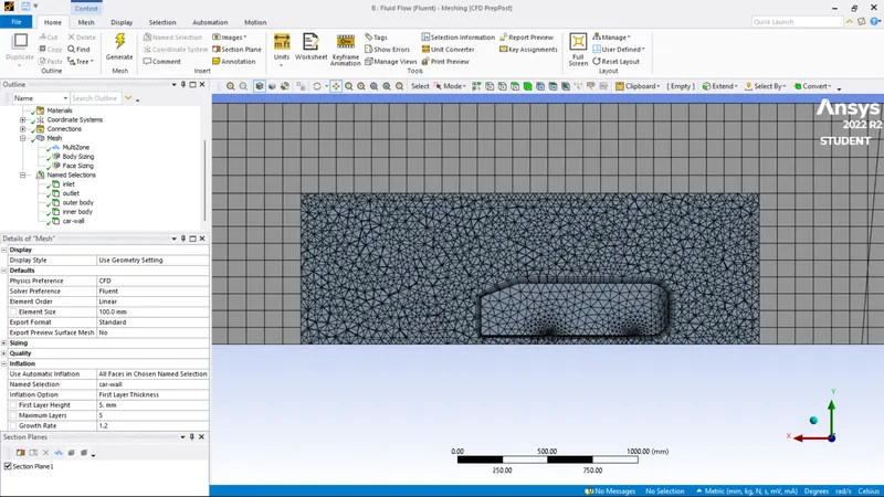
Method

Outside the box, the hexahedral mesh is used. The mesh is of the highest quality and gives higher accuracy.

Sizing: Sizing is is defined as increasing the number of elements by decreasing the element size. The element size of the second closure is 0.05m

Element size for the first enclosure: 0.1m

Maximum size for the first enclosure: 0.1m

Element size for the second enclosure: 50mm (about 1.97 in)

Element size of pillars of Ahmed body: 5mm (about 0.2 in)

Number of elements: 1,92,62

Inflation layer: It is the process of adding layers to the boundary to cover the boundary layer thickness fully.

The first cell height predicted value is 5mm (about 0.2 in)

Inflation layer: 5

Last layer thickness: 15mm (about 0.59 in)

Y+ value: 345

Results

Residual plot

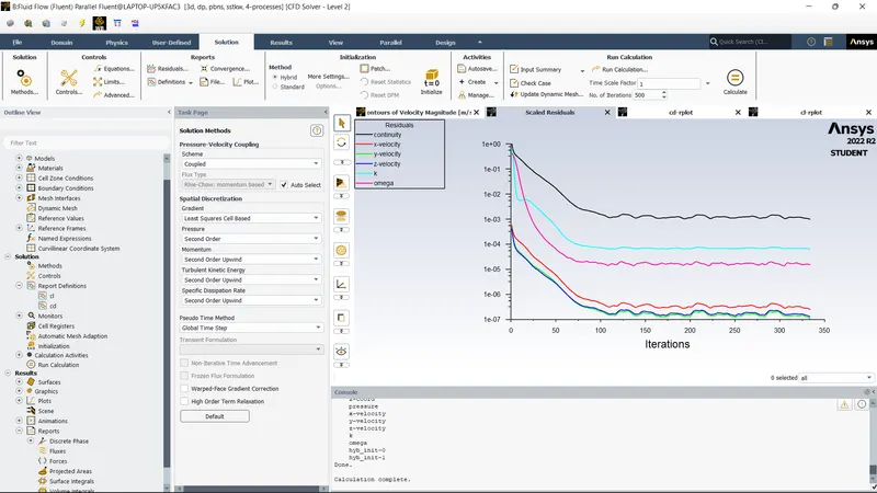
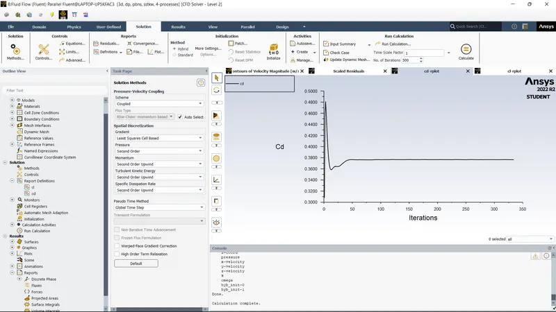
Drag-coefficient plot

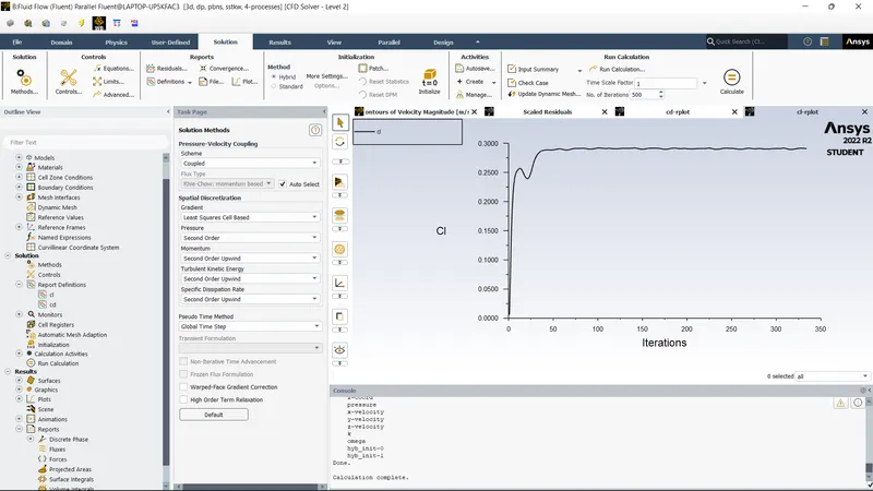
Lift-coefficient plot

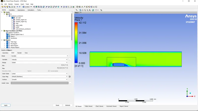
Velocity contour

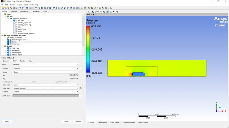
Pressure contour

The vector plot showing the wake region

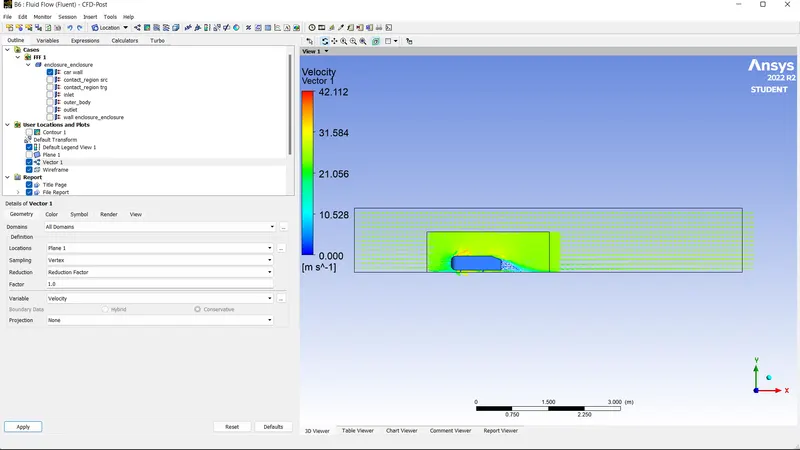
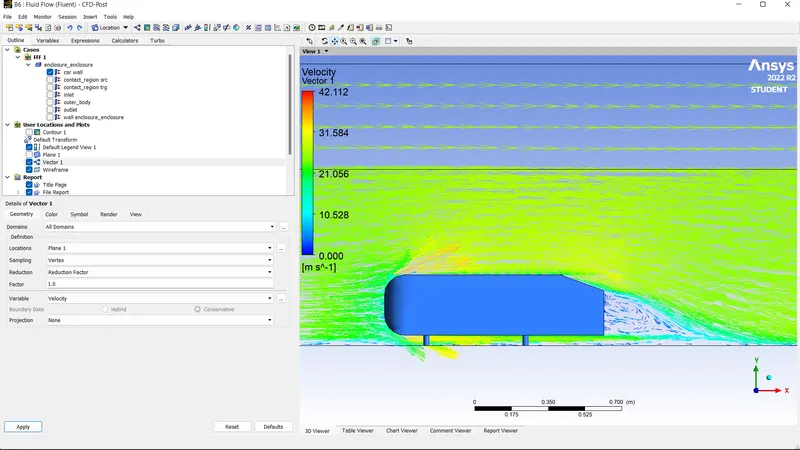
Drag-coefficient	0.376
Lift-coefficient	0.290

Task 2(b): Refinement 2

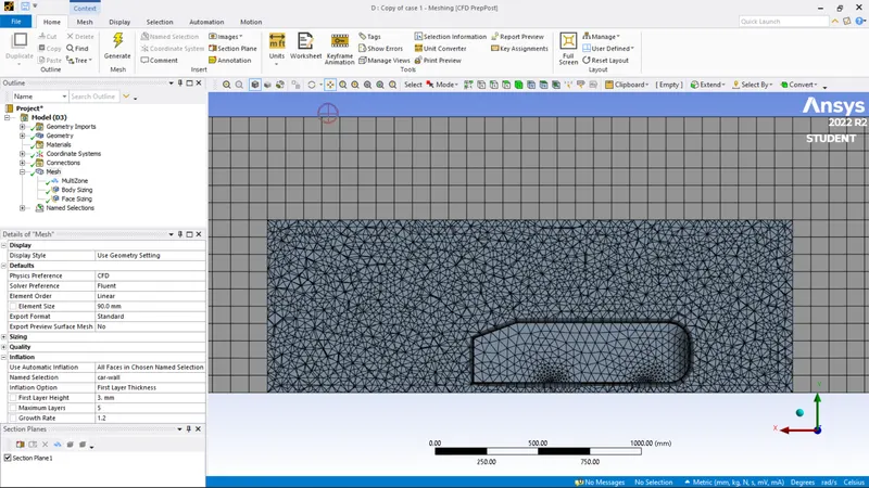
Here The multizone was used for the second area whwere the number of element size for the outer enclosure is taken as 90mm (about 3.54 in) whereas the element size for the inner closure is taken as 45mm (about 1.77 in). Face sizing was implemented for the pillars of Ahmed's body (5mm).

Inflation layer

First layer thickness: 3mm (about 0.12 in)

Number of layers: 10

Last layer thickness: 15.4793m

Number of elements: 253152

The value of y+ is around 207.

Results

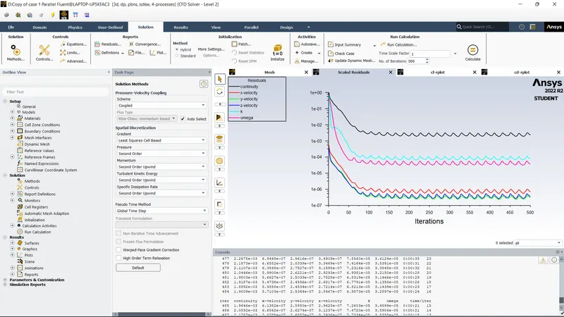
Residual plot

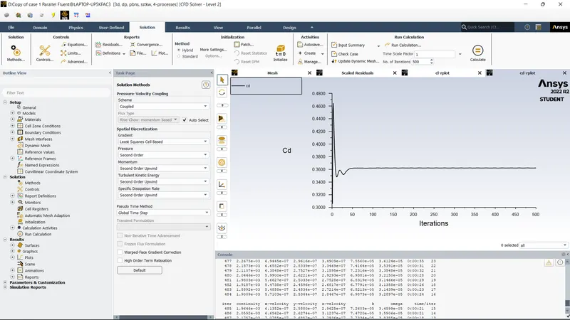
Drag-coefficient plot

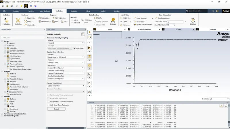
Lift-coefficient plot

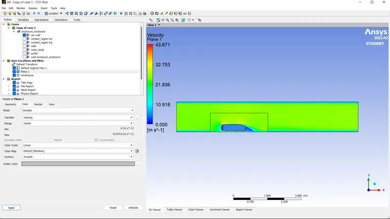
Velocity contour

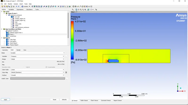
Pressure contour

The vector plot showing the wake region

Drag-coefficient	0.362
Lift-coefficient	0.288

Task 2(c): refinement -3

Element size in the first enclosure: 80mm (about 3.15 in)

Element size in the second enclosure: 40mm (about 1.57 in)

Element size of the bottom leg of Ahmed body: 5mm (about 0.2 in)

Number of inflation layer: 10

First layer thickness: 0.15mm (about 0.01 in)

Last layer thickness: 0.77mm (about 0.03 in)

Number of elements: 348448

Y+: 10

Results

Residual plot

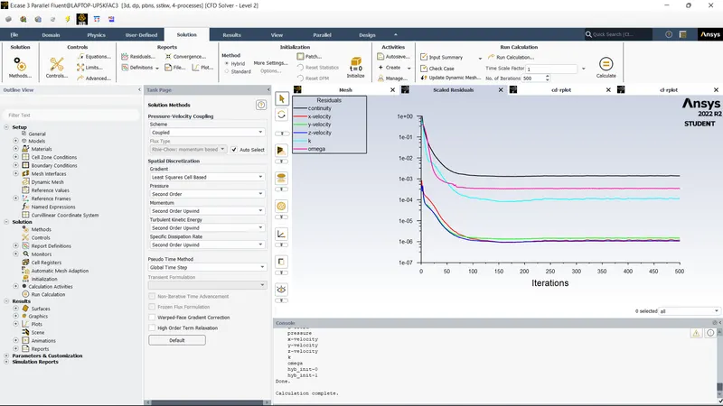
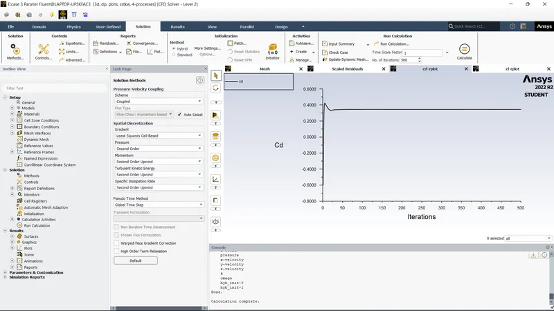
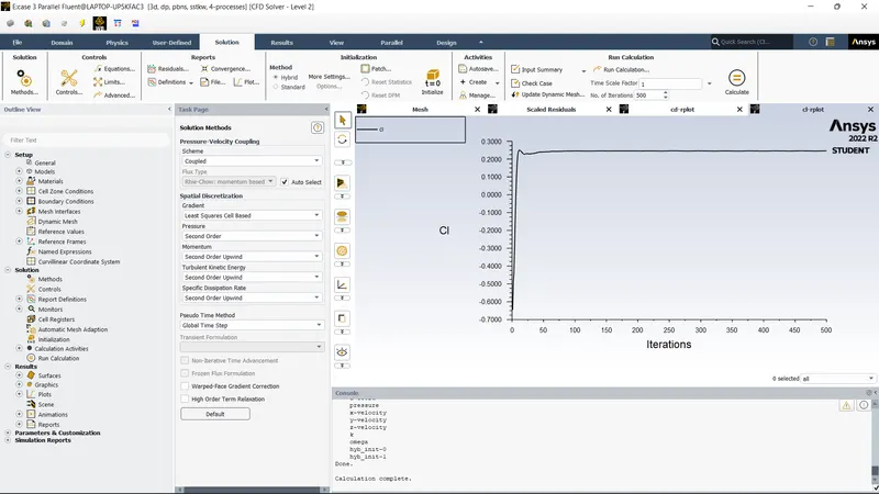
Drag-coefficient plot

Lift-coefficient plot

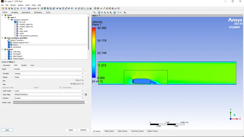
Velocity contour

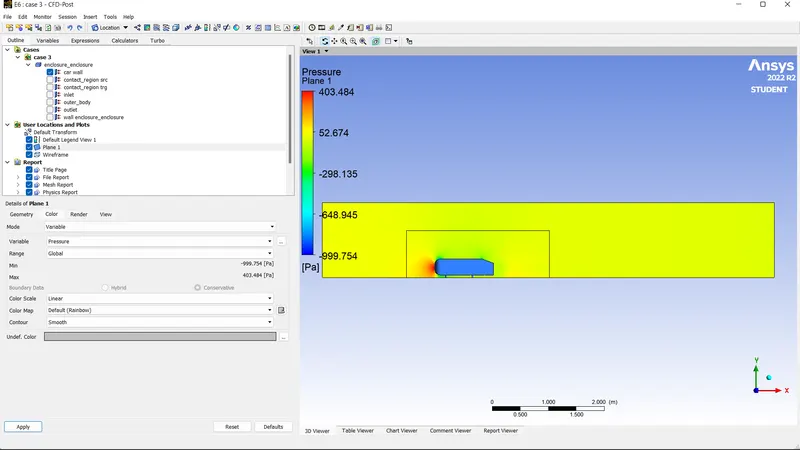
Pressure contour

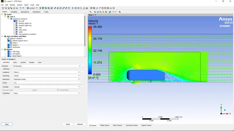
The vector plot showing the wake region

Drag-coefficient	0.343
Lift-coefficient	0.246

Demonstration of grid independence test

Comparison of all cases

Steady-state, Turbulent flow, Density-based, Fluid Material-Air
Grid Independence Test	Turbulence-model	Number of elements	Lift-Coefficient	Drag-Coefficient
Baseline mesh	k−ε	83781	0.225	0.394
First refinement	K−ω SST	192628	0.290	0.376
Second refinement	K−ω SST	253152	0.288	0.362
Third refinement	K−ω SST	348448	0.246	0.343

It can be inferred that the imitation of the experimental result is obtained during the second refinement. Thus, the grid independence test saves a lot of computational time and convergence can be achieved by using smaller cell sizes for calculation.

Conclusion:

• Apart from mesh refinement, convergence depends on the Y+ value, inflation layer, it is advisable to use k−ω SST as the turbulence value because it calculates the values well near the wall.
• The drag coefficient, lift coefficient decreases.
• To determine the drag we can use y+.
• The negative pressure in the wake region is primarily because there is no flow in that region.