Week 3 - External flow simulation over an Ahmed body.

REPORT FOR CHALLENGE-3

Aim : For Lift and Drag coefficient accuracy comparision for the different element sizes after CFD analysis over a Ahmed body, split the given body to symmetry and simulate the flow over the body and calculate the Lift and Drag Coefficients for a given problem using workbench-fluent under steady state for 3 different cases by changing the element size from coarse to fine meshing and discuss the results based on accuracy.

Software Required : Ansys Workbench – Fluid Flow vR2-2022

Hardware Required : Desktop, Keyboard, Mouse, CPU.

Theory:

The Ahmed Body was first created by S.R. Ahmed in his research “Some Salient Features of the Time-Averaged Ground Vehicle Wake” in 1984. Ahmed body is the benchmark model for aerodynamics simulation tools.

The simple geometrical shape has a length of 1.044 meters, height of 0.288 meters, and a width of 0.389 meters. It also has 0.5-meter cylindrical legs attached to the bottom of the body and the rear surface has a slant that falls off at 40 degrees.

Ahmed body represents the simplified ground vehicle geometry of a bluff body type. Its shape is simple enough for accurate flow simulation and retains some important practical features relevant to automobiles body. This model helps us to calculate turbulent flow field around the simple car using the k-epsilon model.

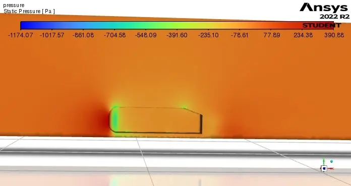
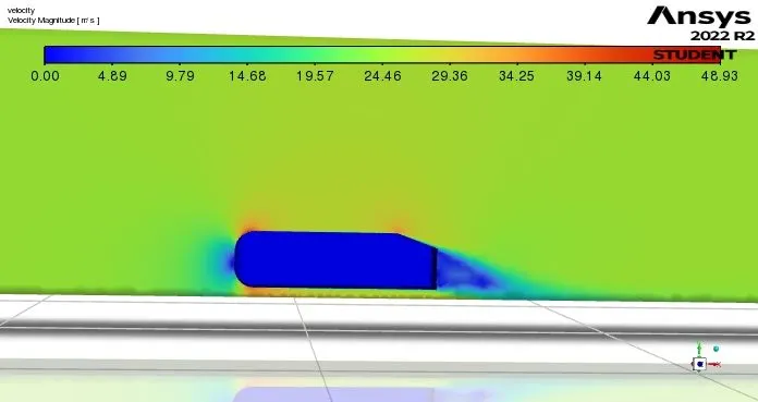
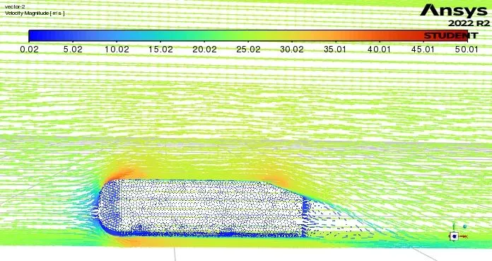
Some of the key characteristics which can be obtained from simulating Ahmed's Body are Velocity Magnitude, Pressure Magnitude, Wake region, Drag Force, Lift Force.

Procedure :

1.Open the Ansys Workbench.

2.Double click or drag the Fluid Flow module.

3.Import the required geometry and do the CAD clean-up.

• Assign the planes for reference.
• Split the geometry by using split-body.
• Create Enclosure-1 and Enclosure-2 with the given suitable dimensions.
• Check for interference and solve.
• Shate the topology.

4.Mesh the geometry with the suitable element size in addition to name all the faces which model have.

• Provide the sizing and method for to assign the different element size and shape for both the enclosures.
• Assign the required mesh size and change mehod to multi-zone.
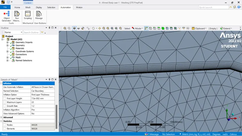
• Create inflation layer with the suitable values.

5.Solve the equations in the set-up and solution block for required result.

• Set 3D, Double Precision and Assign number of cores.
• Set Steady state.
• Change method to Coupled.
• Set Energy on and choose the K-Omega Turbulance model.
• Assign the Material Properties and Boundary conditions.
• Check and assign all the Reference values properly.
• Create definition plots for CL,CD.
• Create Contours.
• Initialize and Calculate.
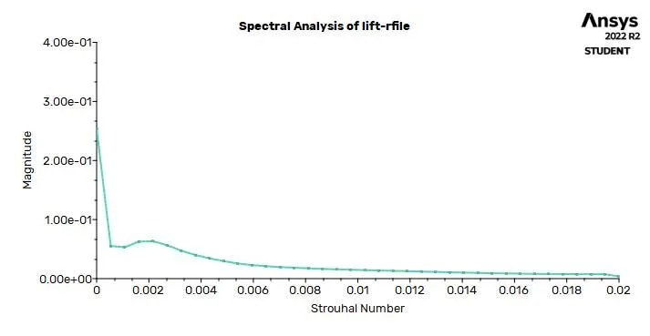
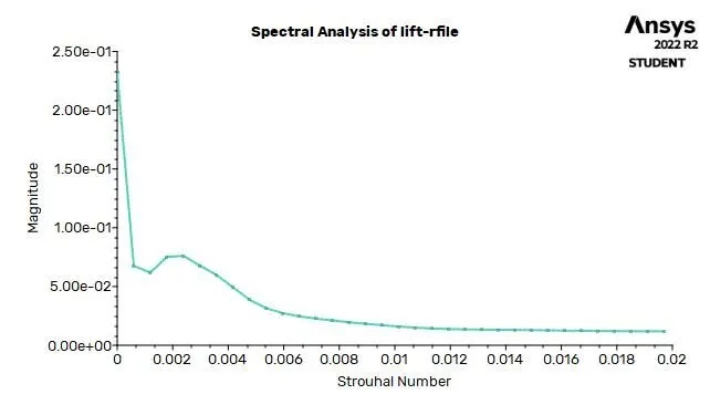
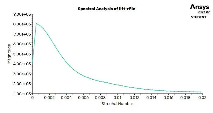
• Plot the strouhal number.

6.Then do the post-processing in the CFD solver in the result block.

7.Save and close the file.

Observations :

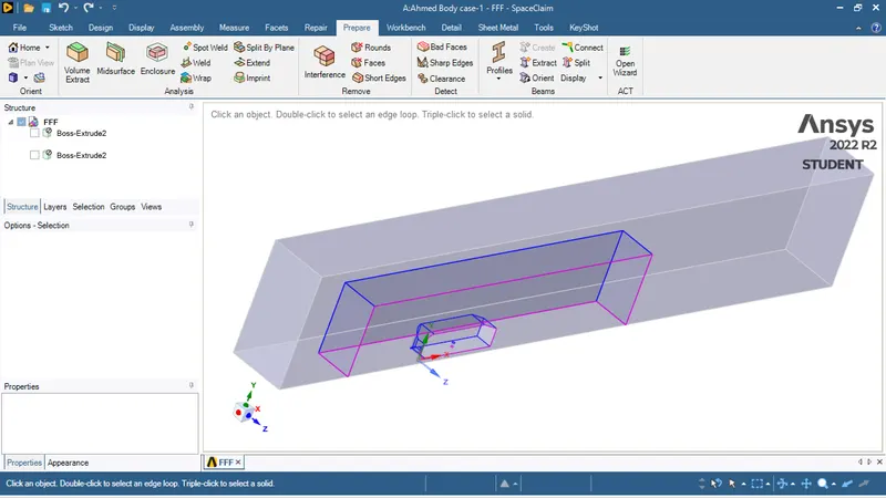
Geometry:

-Model to be Analize after Cad clean-up.

Mesh Details:

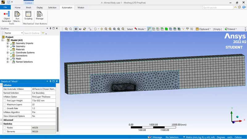
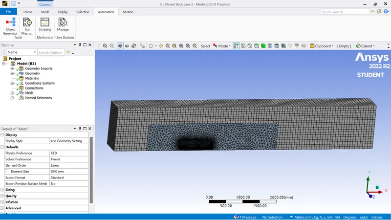
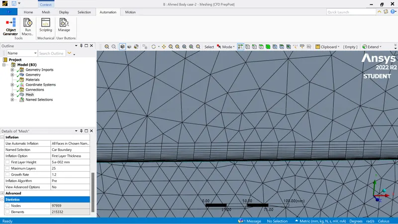
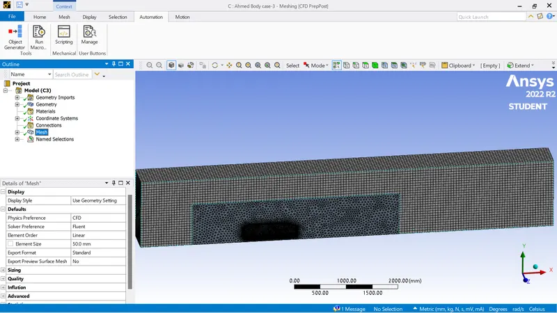
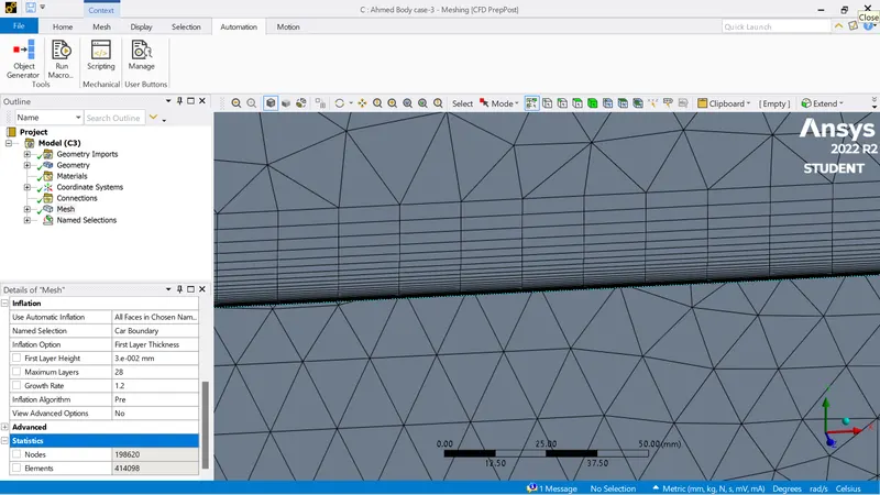
On the consideration of the accuracy of the result, we worked on the concept of independent grid generation. So, we analysed the given Ahmed Body in 3 different cases which are on the basis of the three different mesh methods which are Coarse, Medium and Fine mesh and all the mesh details were given below,

Case	Size	Splitting	Inflation	Layer	Detais			Total No.of Elements
-	Assigned Domain volume cell size(mm)	Car Volume Cell size (mm)	Y+	Boundary layer thickness (mm)	First layer thickness (mm)	Growth Rate	No.of Layers	-
Coarse	120	30	1	21.922	0.075	1.2	22	96,526
Medium	80	20	1	21.922	0.050	1.2	25	2,15,332
Fine	50	15	1	21.922	0.030	1.2	28	4,14,098

1.Coarse Mesh:

2.Medium Mesh:

3.Fine Mesh:

Reference values:

Density	1.225kg/m^3
Velocity	25m/s
Area	0.0657m^2
Viscosity	0.05N-s/m^2

Boundary Conditions:

The entire analysis of the given Ahmed Body was done in the flow field having the velocity of 25m/s.

Solution Status:

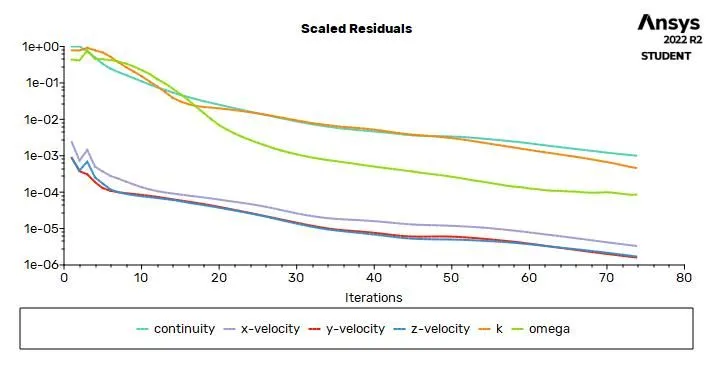
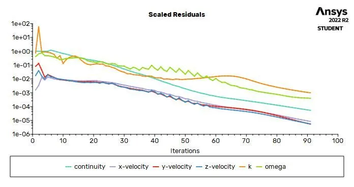
We analyzed the given body in 3 cases such as Coarse, Medium and Fine Meshing based on the No.of Elements.

Case	Total iterations of convergence	Time taken (sec)
1.	74	63.09
2.	67	116.44
3.	91	319.75

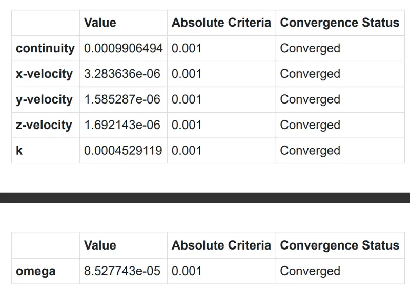
Case-1:

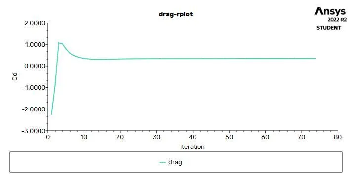
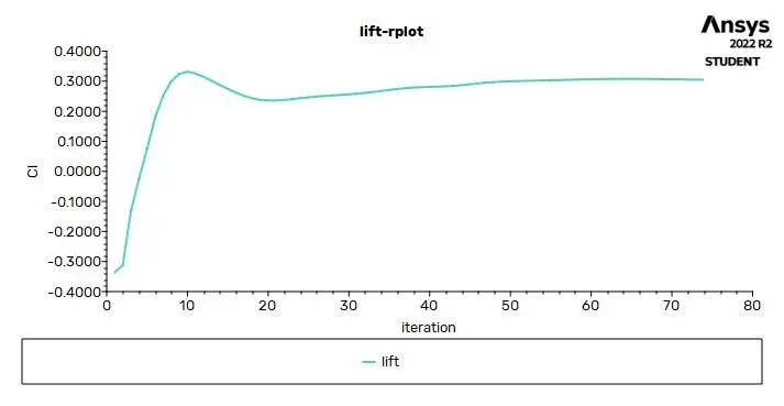
-After the required equations solved, tabulated the results that were obtained.

Plots and Contours:

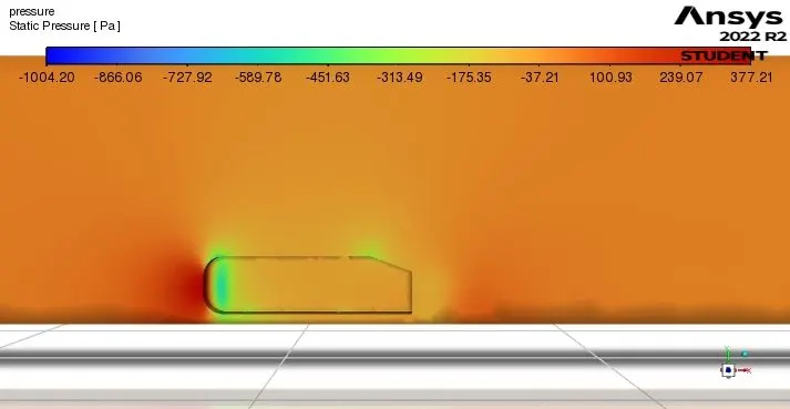
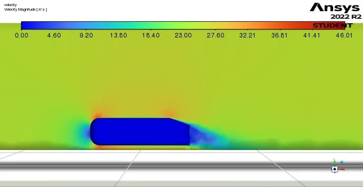
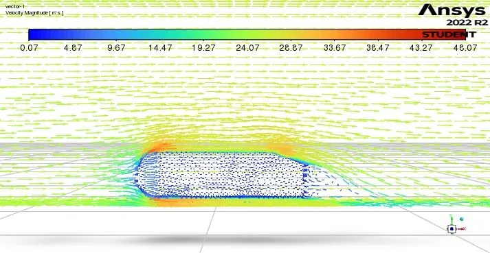
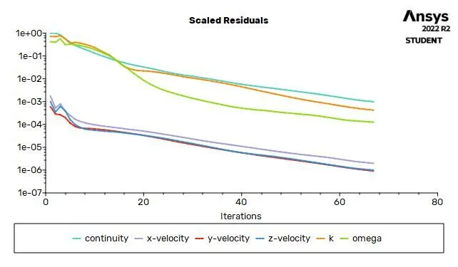
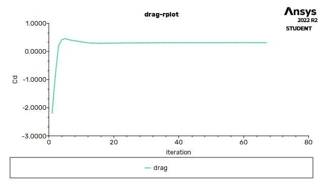
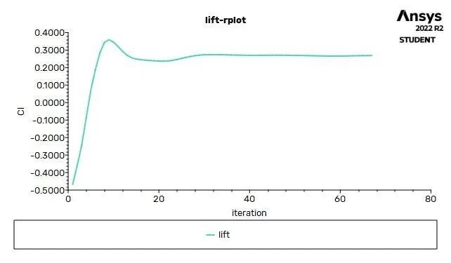
Case-2:

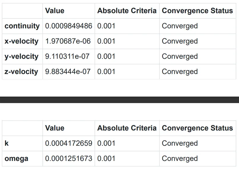
-After the required equations solved, tabulated the results that were obtained.

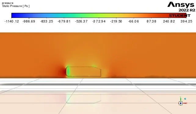
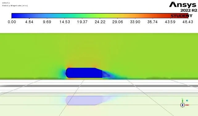
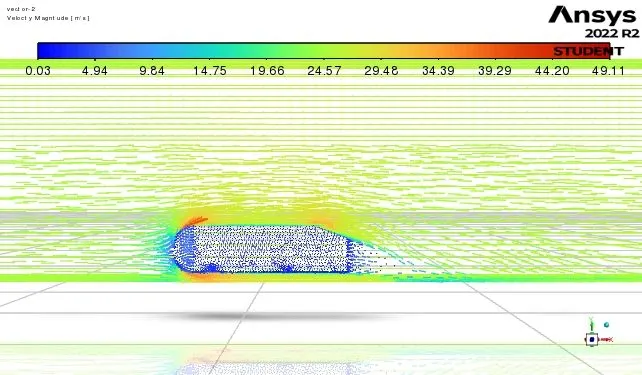
Plots and Contours:

Case-3:

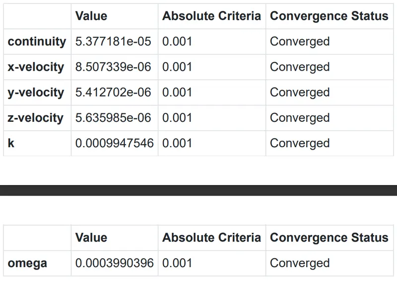
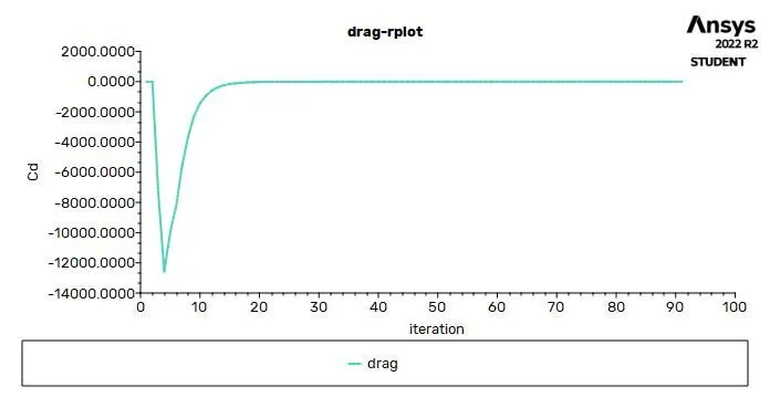
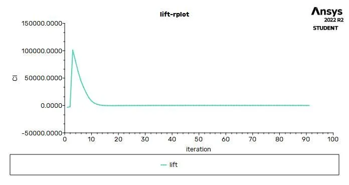
-After the required equations solved, tabulated the results that were obtained.

Plots and Contours:

Precautions :

1.Carefully solve the problem.

2.Choose the suitable methods carefully for to get the desired results.

3.Note down the values carefully which are required for theoretical calculations.

Result:

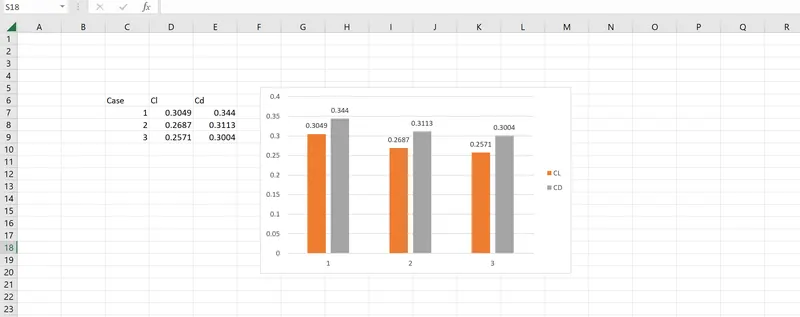
Lift and Drag coefficients for 3 different element sizes was given below,

Case	Total No.of Elements	CL	CD
Coarse	96,526	0.3049	0.3440
Medium	2,15,332	0.2687	0.3113
Fine	4,14,098	0.2571	0.3004

Accuracy Comparision Graph for lift coefficient and drag coefficient for 3 different cases.

Conclusion:

When the fluid is passing over a body there are many changes happens in the properties since attaching to detaching to the body. Which means properties of the fluid is not constant if there is any obstacle present in the way of fluid direction. There will be change in the Pressure, Velocity, etc,.Due to the pressure and velocity change while contact with the body, there will be some forces are generated like lift, drag, etc,.While detaching the fluid from the body, eddys or vortexes forms behind the body to certain distance.

The flow around a bluff body produces a regular pattern of alternating vortices. These vortices produce a sinusoidal force acting on the body perpendicular to the flow.For very small Reynolds Number, the flow is completely laminar around the cylinder, with no recirculation and no instability.

For larger Reynolds numbers, a recirculation zone appears behind the obstacle. More precisely, two eddies with opposite signs appear just behind the cylinder and remain close to it.For larger Reynolds numbers, these eddies are unstable and successively leave the body to propagate in the wake. Increase in the velocity leads to increase in the Reynolds number, which leads to indrease in the vortex shedding and for every increase in the reynolds number leads to increase in the Strouhal Number.

For to get the desired results accurately, we need the fine mesh. After studied all the cases we can conclude that mesh sizing is the major thing for to get the accurate results after doing the CFD analysis over any body in any fluid properties.