External flow simulation over an Ahmed body.
Aim: Performing external fluid flow simulation over an Ahmed body.
Objective:
- To understand the requirements of setting up an external fluid flow domain to obtain solution by CFD.
- To understand the importance of standard wind tunnel models (here, Ahmed body).
- To understand the requirements for implementation of given domain in commercial CFD codes (here, Ansys Fluent).
- To understand the concept of multizonal mesh refinement and usage of non-dimensionalised parameters such as y+ value.
Introduction:
What is Ahmed body, and why is it important?
Automobiles experience opposition to its motion, owing to the drag force acting on it. The load offered by this resistance is fulfilled by the automobile's engine. Therefore, to obtain better fuel economy, it is essential that this drag force is minimised. However, to model and study the actual vehicle is difficult, owing to the complexity in the external structure of a vehicle and thereby obtain the drag computationally.
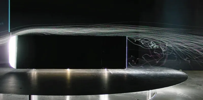
The Ahmed Body was first created by S.R. Ahmed in his research “Some Salient Features of the Time-Averaged Ground Vehicle Wake” in 1984. Ahmed body is the benchmark model for aerodynamics simulation tools. The geometry of Ahmed body is simple enough to perform computations while it maintains a car like geometry. Three main features were seen in the wake:
- The recirculation region that is formed as the flow separates at the top of the vertical back surface of the model
- The recirculation region that is formed due to the separation at the base of the model.
- The c-pillar vortices that form as the vorticity in the side boundary layers roll up over the slant edges.
 |
Explain the reason for the negative pressure in the wake region.
Refer conclusion (pt. 4)
Explain the significance of the point of separation.
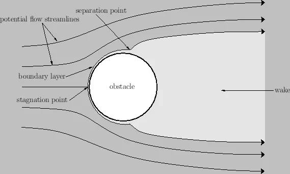
A boundary layer exists, when there is a relative motion between the fluid and a body immersed in this fluid. Thickness of this boundary is minimum at the fluid stagnation point and steadily increases along the length (surface) of the body. However, the boundary layer gets separated at some distance, causing high energy losses and formation of wake. This phenomenon is known as boundary layer separation.
This boundary layer separation is observed to take place at a point where adverse pressure gradient exists, and this point is therefore termed as the point of separation.
 |
Workflow:
- Preparing the geometry
- Generate mesh for the geometry
- Setting up the solver
- Setting up the solution monitors
- Post-processing to observe the results
Ansys Fluent:
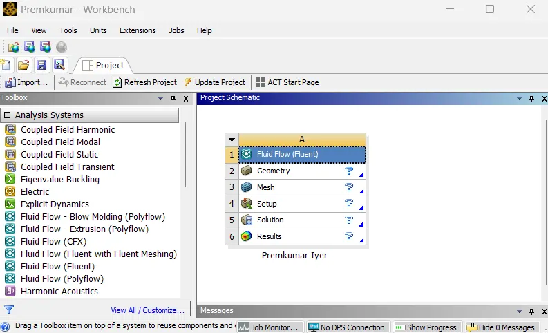 |
In the Ansys workbench project window, Fluid Flow (Fluent) is dropped into the workspace.
Preparing the geometry:
The computational domain followed for the simulation is as shown below:
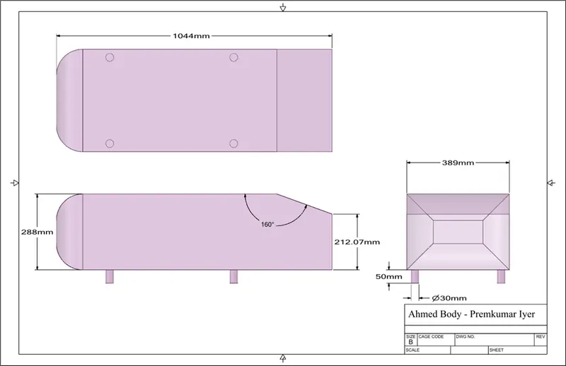 |
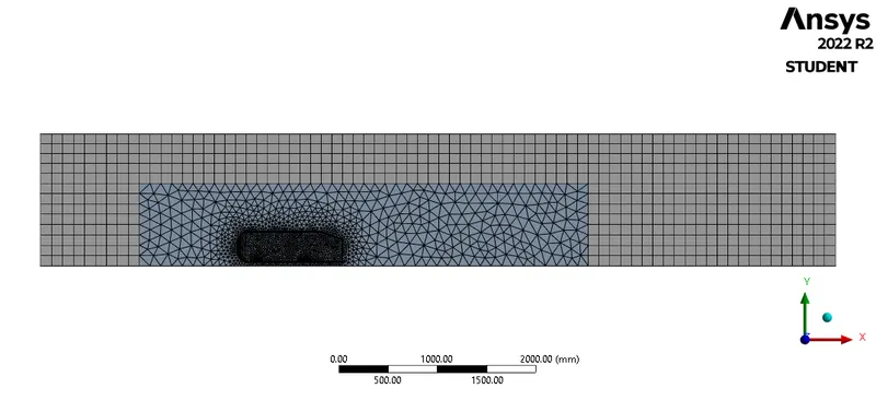
The computational domain, as shown (provided as a STEP file) is imported in SpaceClaim. Since, the body is symmetrical about XY plane (as per the reference axis), the body is split into two halves along the plane of which, one part is retained. This helps reduce the computational load (by applying symmetric boundary condition). Further, since the flow is happening over the Ahmed body, an enclosure is defined for the the fluid (here, air) to flow. And, since, the important changes in the fluid is observed at distance just before the frontal surface and the wake region formed behind the body, another enclosing surface is defined. This is done so that the mesh in free flow regions are coarse and in the important areas are fine enough to capture the necessary details with minimum errors and computational resources.
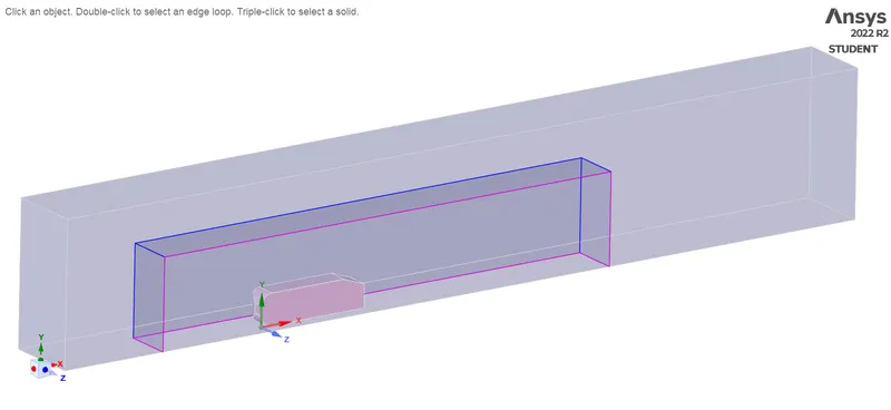 |
However, when the second enclosure is introduced, the meshing has errors (the mesh overlaps each other in the second zone). This happens because there exists area between the "original" enclosure and the second enclosure which is co-shared by them, and hence in SpaceClaim, these regions are selected and then the topology of these areas is shared by checking the interference and rectifying it (this option is present under the prepare tab).
Generating mesh:
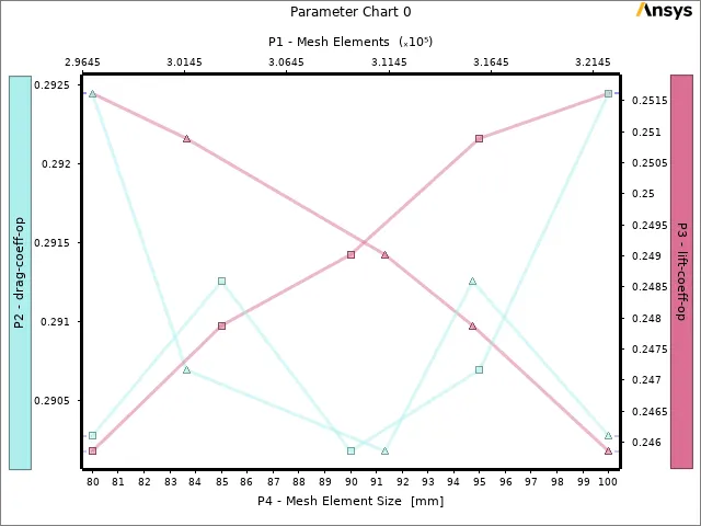
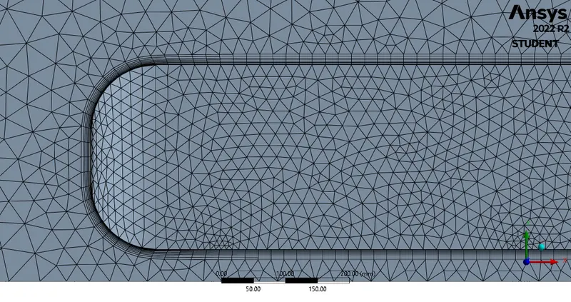
Meshing is the process, wherein the geometry is divided into smaller parts which are known as elements, so that the iterative solver can solve the governing equations across the domain. In the meshing utility, a baseline mesh of element size 100mm (randomly chosen) is provided. Further, the method of meshing is inserted as "multizone" and thereby, a hexahedral mesh in enclsoure and tetrahedral mesh in refined region is observed. Since, the boundary layer formed over the Ahmed body has to be captured, and therefore face sizing with 20mm element size was provided. Moreover, the cylinderical legs of the body loses its cylindericity, and therfore face sizing of 20mm is provided to this too. An inflation (randomly provided) is applied based on an assumed y+ value (of 30). The case was set by parametric study, wherein the element size of mesh was the input parameter and the coefficient of drag and lift were the output parameters. By this, an optimised grid was chosen, but the coefficient values were inaccurate due to incorrect y+value, which is cross-verified in Fluent (Report definition>Turbulence>Y-plus). The y+ is reported to around 44.12981.
 |
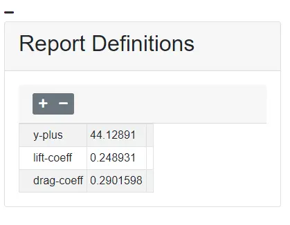 |
| Parametric Chart | Y-plus value |
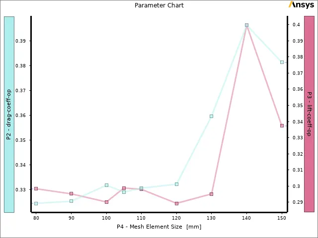
And, thus, modifications in the inflation layer thickness was done taking this into account, and, thus, we have:
 |
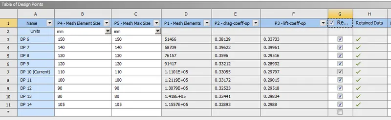 |
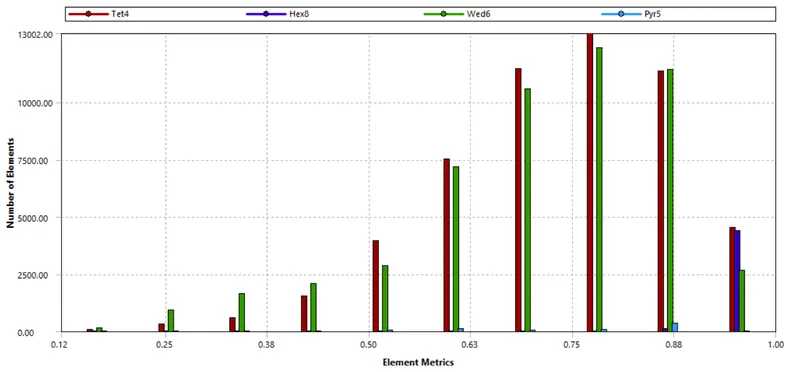
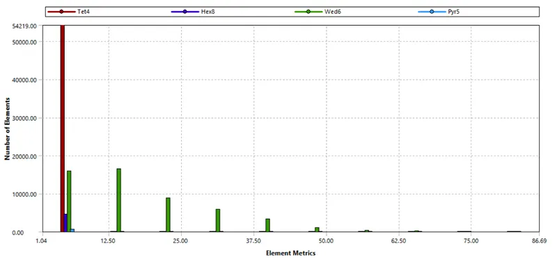
From the above, the it was concluded that 110mm of mesh element size is optimum for our study. And, thereby, the generated mesh and its mesh metrics are as shown below:
| Orthogonal Quality | Aspect Ratio |
 |
 |
 |
|
 |
|
For implementing the boundary conditions, the "boundaries" must be clearly defined. To do so, the mesh utility itself has a tool; named selections. By selecting the respective faces and surfaces, the velocity inlet, the pressure outlet, symmetry and the car wall was defined.
Seting up the solver:
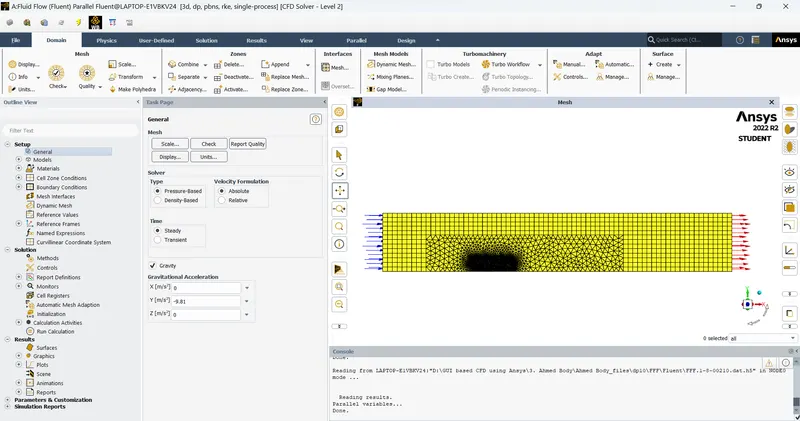 |
An important part of a CFD simulation, the setup for solver is done to obtain the solution. Firstly, the units of important parameters are set to desired units (preferably SI units). In the models tab, in the viscous models, `k-epsilon` realizable with enhanced wall functions is chosen. The fluid zone contains air, and the default properties from the Fluent database is utilised. The only boundary condition that we need to provide is the inlet velocity (which is set as 25m/s), rest everything is left untouched. The reference values are altered with respect to the inlet. The projected area of the car body is evaluated from the option (by the same name) available under the results tab.
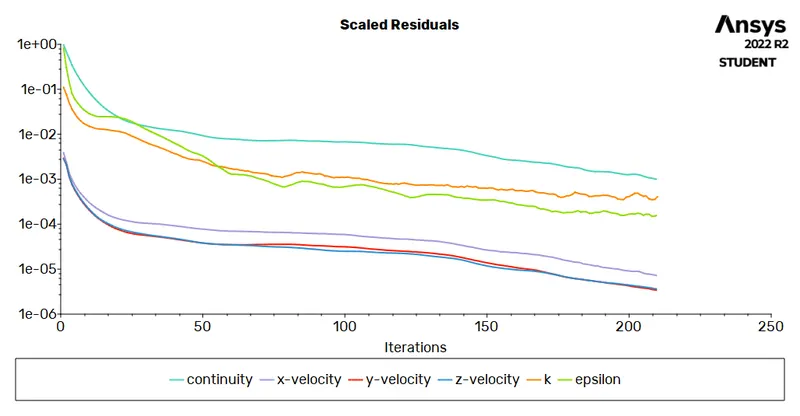
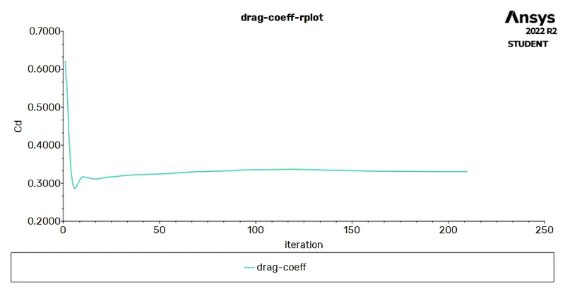
The pressure-velocity coupling is set to SIMPLE and the momentum and pressure are set to second order discretisation. Report definitions are set to capture the coefficient of drag and lift over the car body surface. The corresponding plots along with the residual plots are saved. Hybrid initialization is used to initiate the problem, thereafter, 500 iterations are provided for the solver.
Post-processing (Results):
 |
 |
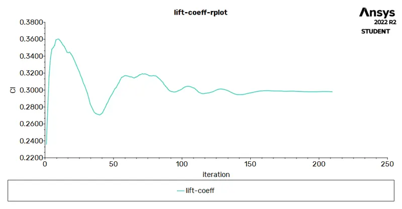 |
| Residuals Plot | Drag Coefficient - 0.33055 | Lift Coefficient - 0.29797 |
 |
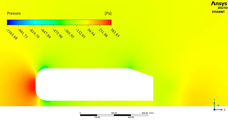 |
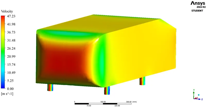
| Pressure on the car body | Pressure contour |
 |
|
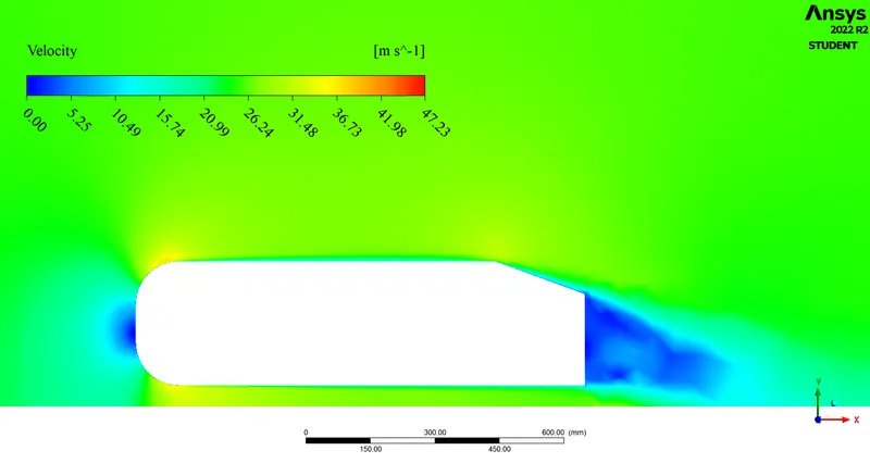
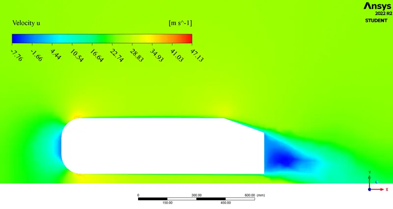
| Velocity Contour | |
 |
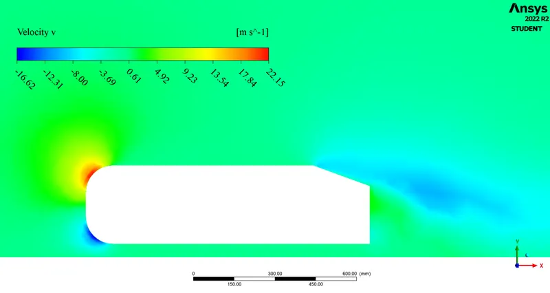 |
| x-velocity contour | y-velocity contour |
 |
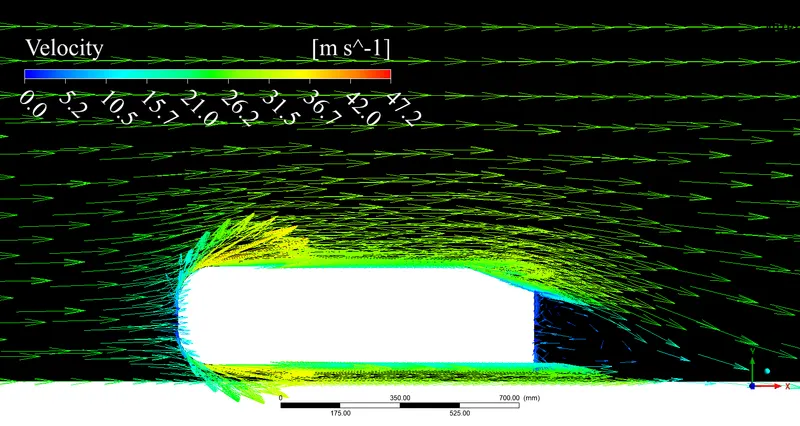 |
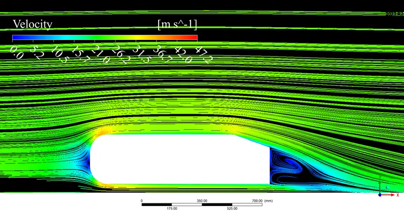
| Streamlines | Velocity Vector |
Conclusion(s):
- The project involved study of a standard wind tunnel model, the Ahmed body and a grid indepedence study is done by parameterizing the mesh element size, and consequently, the coefficient of drag and lift were computed by careful investigation and selection of inflation layer thickness as dictated by the y+ value.
- The pressure rises in the frontal area of the car body. This is because, air after striking the face of the car body, becomes stagnant and thereby, converting the kinetic energy to pressure energy. However, over the curvature of frontal area, the pressure is observed to be dropping. This is because the fluid is accelerated here, i.e., a change in direction is experienced by the air (as evident from the streamline and velocity vectors).
- The x-velocity contour clearly illustrates how the flow recirculation in the wake region occurs and the y-velocity contour illustatrates the divergence of flow, when the air strikes the face of the car body. The streamline and vector plots are very well aligned with this flow description.
- In the rear section of the car body, the boundary layer follows the surface and detaches after the slant region. This detachment causes a drop in energy (and thereby pressure) and the reference pressure for this study is standard atmospheric pressure (1atm). Moreover, in this region, due to the adverse pressure gradient, flow circulation takes place. Hence, in the rear (where wake is formed), the static as well as dyanmic pressure is therefore reduced, thus the pressure in this region is negative. This wake formation also increases the drag force due to the pressure drag.
- The results show high degree of coherence with the literature being referred for this problem, and hence, the solution is validated.
References:
- Introduction to GUI based CFD using Ansys Fluent - Course provided by Skill-Lync
- Ansys Inc.
- Volupe Engineering Software: y+ calculator
- Supporting Material: Flow and Turbulence Structures in the Wake of a Simplified Car Model
- Supporting Material: Experiments and Numerical Simulations on the Aerodynamics of the Ahmed Body
- Supporting Material: A-TO-Z GUIDE TO THERMODYNAMICS, HEAT & MASS TRANSFER, AND FLUIDS ENGINEERING
- Supporting Material: Studying the Airflow Over a Car Using an Ahmed Body
- Supporting Material: Boundary Layer Separation
- Supporting Material: Investigation of relationship between drag and lift coefficients for a generic car model
- Supporting Material: Fluid Mechanics - Frank M White
- Supporting Material: Fluid Mechanics: Fundamentals an Applications - Y Cengel and J Cimbala