Week 3 - External flow simulation over an Ahmed body.

Aim:

To Simulate the external flow over an Ahmed Body. And we can run the simulation by considering the only half body. To run the simulation for the velocity of 25 m/sec with the default air properties in fluent.

Objective:

In this challenge we have to do simulation of the flow over a circular cylinder and then we have to get some pressure, velocity, vectors and streamline plots and contours from the simulation. Below are the objectives of this challenge we have to follow these steps.

Q1. Describe Ahmed's body and its importance.

Q2. Explain the reason for the negative pressure in the wake region.

Q3. Explain the significance of the point of separation.

1. Velocity and pressure contours.
2. The drag coefficient plot for a refined case. (For velocity of 25m/sec, the drag coefficient should be around 0.33).
3. The vector plot clearly showing the wake region.
4. Perform the grid independency test and provide the values of drag and lift with each case.

Ahmed body:

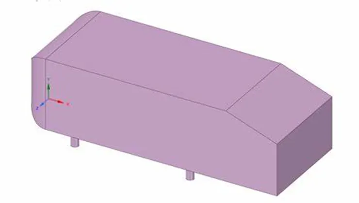
Ahmed body is a simplified car model geometry. Ahmed body is used to capture the basic flow characteristics of an automobile. CFD is used to study the aerodynamic behaviour of Ahmed body.

The Ahmed body is a benchmark model widely used in the automotive industry for validating simulation tools. The Ahmed body shape is simple enough to model, while maintaining car-like geometry features.

Ahmed body was developed by S.R. Ahmed & presented in his research paper “Some Salient Features of the Time-Averaged Ground Vehicle Wake” in 1984. This body is used as a generic car body because it captures all the essential flow features around an automobile and is easy to model.

The simple model makes meshing easier, reduces the computational power required and the time taken to run the simulations. Hence the body is widely used by researchers & engineers to validate their numerical model or CFD codes and sometimes without even wind tunnel testing as vast experimental data is already available (for different scale models of Ahmed body) from validation studies over the years.

Negative pressure in the wake region:

• Negative pressure in the wake region the fluid as it flows Ahmed body there would be stagnation of air particles at the front of the Ahmed body and pressure would be more which can be seen from the pressure contour, then there would be gradual increase in the acceleration of the air particles till the start of the slant angle
• Reason for negative pressure in the wake region: The path lines showing the exact circular motion or vorticity generation just at the rear end of the car. The separation takes two regions of distribution. One at the upper part of the rear and the other at the lower part of the rear end.
• The flow around the vehicle is characterized by high turbulent and three-dimensional flow separations as well as there is a growing need for more insight into the physical features of these dynamical flows. The Ahmed Body is a simplified car, used in the automotive field to investigate the flow analysis and find the wake flow around the body.

Point of separation:

The rear slant angle of the Ahmed body has a considerable effect on the flow separation at the rear end and the 25-degree configuration, particularly, is the one of the critical cases where flow experiences both flow separation and reattachment over the rear slant surface.

The flow separation happens at different points for a body based on the type of flow, basically, Laminar or Turbulent. For the laminar flow, the flow separation happens quickly resulting in minimal shear drag and a large pressure drag which forms a wake region (low pressure) behind the body, while for the turbulent flow, the flow separation is delayed causing minimal pressure

Procedure to simulate the ahmed body:

• First we importing the ahmed body in space claim geometry by drag the file and pull into the sketch.
• After in above tool bar under prepare section enclosure option selecting and unenabling the symmetry option giving the dimension we creating the enclosure to the ahmed body with two enclosure and we supress the ahmed body.
• two enclosure because to reduce the number of mesh element.
• After the creating enclosure we split the body by using split option which option is there under prepare section by selecting plane like which make equal half we split the body.
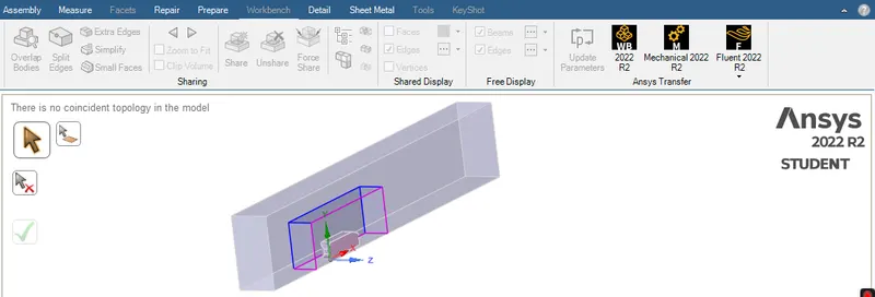
• After spliting the body we do the interference, we do interference because if we don't do the interference the air doesn't flow inside the enclosure of the inner enclosure.
• After doing the interference we do the topo share this we do because to match the outer enclosure mesh to the inner enclosure mesh
• Then doing this all geometry cleanup we open the mesh window and performing mesh by giving some size based on problem statement, For to reduce mesh size of inner enclosure we use sizing option which is there when right click on the 'mesh' sizing option we can see by selecting that we give mesh to the inner enclosure but before that we hiding the outer enclosure by using face option we selecting outer enclosure and click the F8 button, Similarly for ahmed body foot using sizing option by selecting foot face we giving the mesh size over there Then last we generating the mesh
• Then we give the naming for inlet, outlet, symmetry and carwall this we do by selecting face and clicking shortcut key 'N' option
• Then next to the name selection we giving the inflation layer by calculating Yplus and giving this Yplus value as firstlayer thickness in the option and selcting car wall we create the inflation to the car wall
• So like this we meshing with different sizing we studing the three cases of simulation.
• After the mesh to run the simulation we open the setup window, In set up window under viscous option we selecting the k-epsilon model and enhance wall treatment option.
• And we take out the drag and lift graph sheet from under the report definition option
• Next we giving the boundary condition to the inlet and outlet, Then in reference value we given where flow to compute from and in reference value we giving the frontal area value of the ahmed body and the length value
• next we initializing the problem and run the simulation for the particular iteration where the solution is get to converge.
• Lastly we taking out the results from solution and from post processing.
• Note: To take yplus value in report option we open the surface integral task page in that report type we select average weightage area option, In field variable we select the turbulence option and the wall yplus option and last we selecting the body of what body yplus we want.

Step 1: Geometry

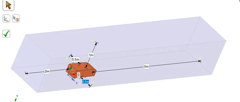
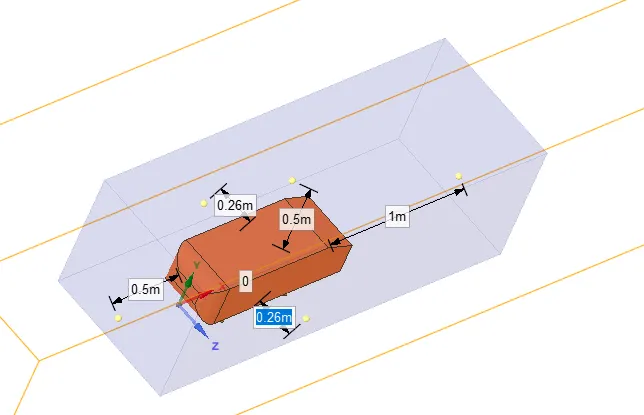
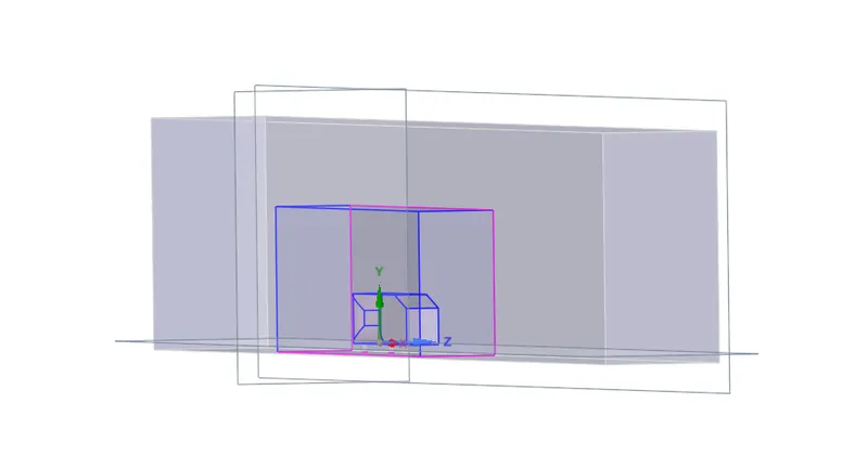
First, we have to upload the given model (Ahmed body) in ANSYS fluent . next step is we have to create two enclosers for given Ahmed body.

Front (m) Back (m) Top (m) Bottom (m) Side (m)

Outer enclosure 2 5 1 0 0.5

Inner enclosure 0.5 1 0.5 0 0.25

Step 2: Meshing

Case (Element Outer Enclosure Inner enclosure Car wall

size) in (mm)

Case 1 250 100 5

Case 2 100 50 3

Case 3 80 45 3

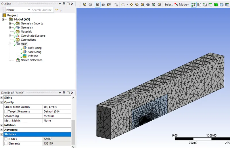
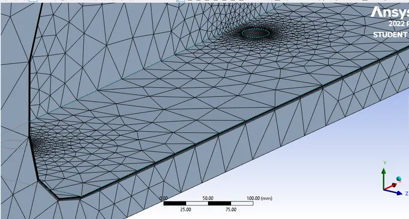
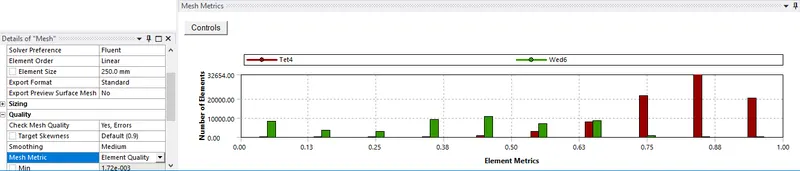
mesh of the three cases

case 1:-

case 2:-

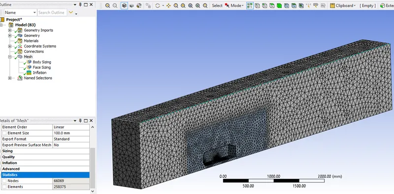
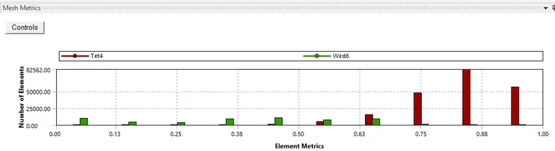
case 3:-

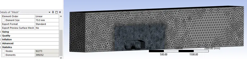
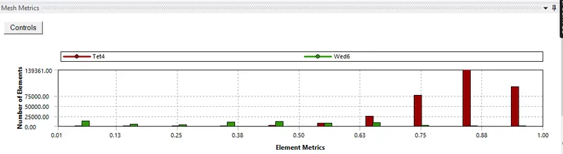
set-up:

setup and solutoin process already mentioned in above in the procedure.

Results:

Finally, we just do right click and open the Result option it will show the Post processor. In the result tab we have to see the default view is a wireframe model, we can create a plane in XY to view contours and vectors. Selecting the Vector and selecting the plane creates a velocity vector. We have cretae the streamline contours three cases for velocity vector by using streamline option. And then we should create the lines at distance of 1.05 m, 1.5 m, 2 m away from the tail of the car to study the velocity chart on the same. Plots can be created using the CHART option. For Case 1, 2and Case 3, we shall repeat the same except for changing the grid size in meshing step. We can simply DUPLICATE case 2 fluent file and edit in it.

scaled residual plot, drag coefficient plot, lift coefficient for three cases:

case1:-

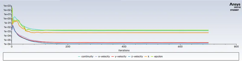
scaled residuals

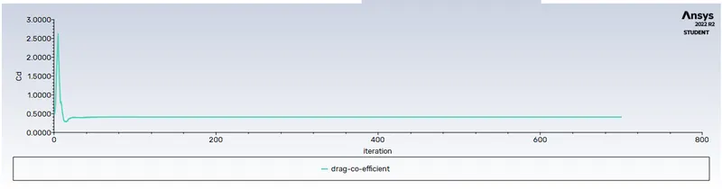
drag coefficient plot

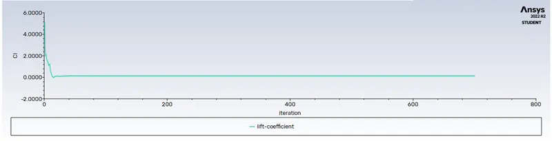
lift coefficient plot

case2:-

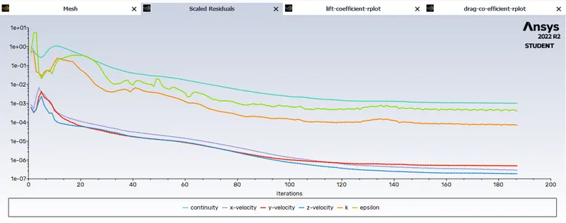
scaled residuals

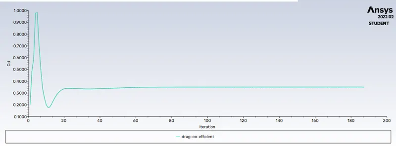
drag coefficient plot

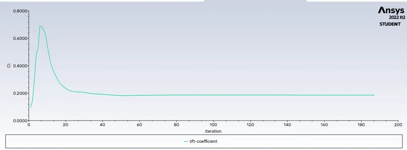
lift coefficient plot

case3:-

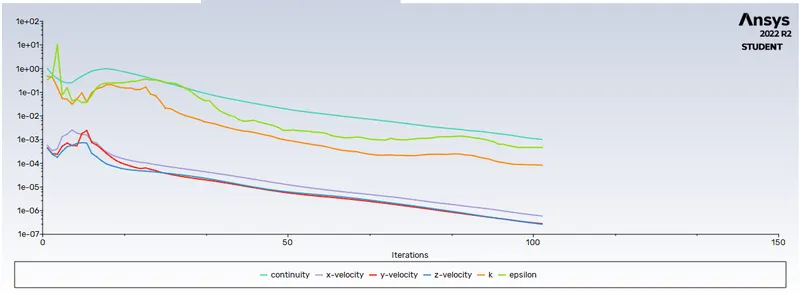
scaled residuals

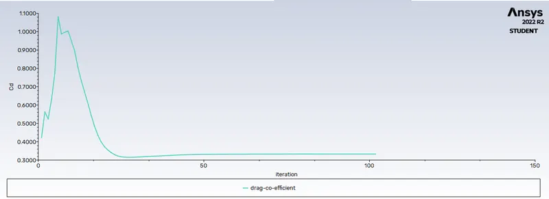
drag coefficient plot

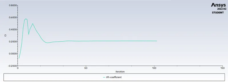
lift coefficient plot

contour plots for the three cases:

1case:-

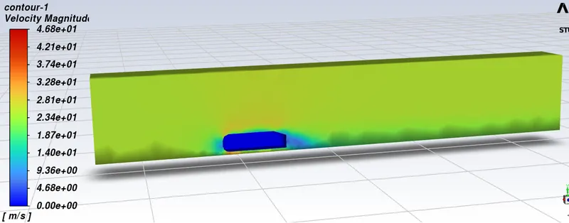
velocity contour

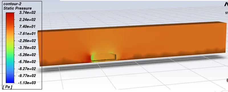
pressure contour

case2:-

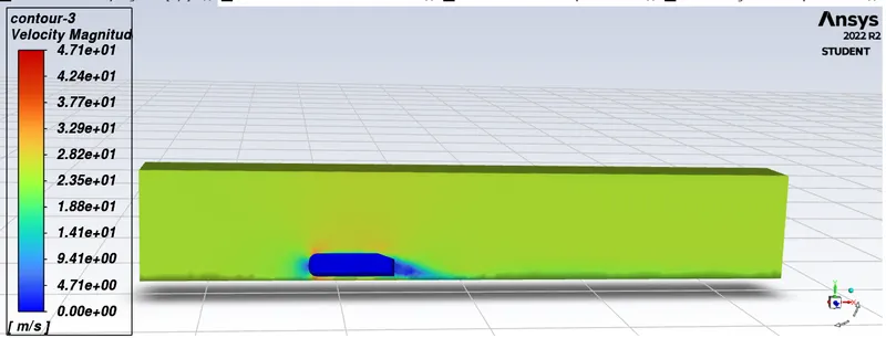
velocity contour

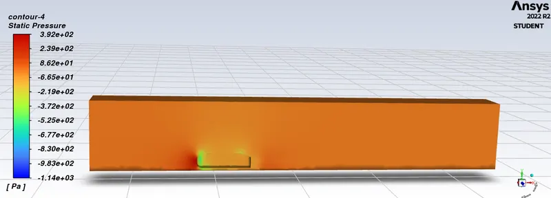
pressure contour

case3:-

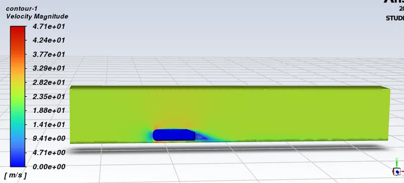
velocity contour

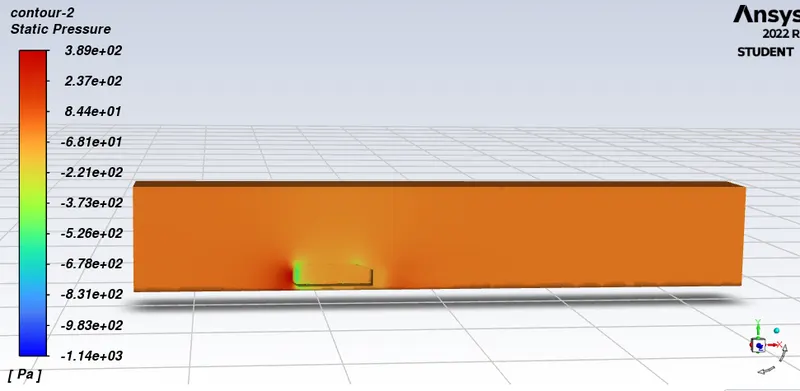
pressure contour

• By looking above image of three case study third case study gives more accurate result than first two case.
• By this we conclude finer the mesh more the accurate result.

Conclusion:

The results of all 3 cases, and we got the drag coefficient and lift coefficient values.

Case 1 Case 2 Case 3

Outer enclosure 250 100 80

Inner enclosure 100 50 45

Car wall 5 3 3

Drag coefficient 0.425 0.359 0.334

Lift coefficient 0.203 0.240 0.223

So by following above procedure the simulation run successfully.

References:

https://www.researchgate.net/publication/330383775_Experiments_and_numerical_simulations_on_the_aerodynamics_of_the_Ahmed_body

https://flowvision.ru/images/articles/2020/Add_files/Ahmed_1984.pdf