Week 3.5 - Deriving 4th order approximation of a 2nd order derivative using Taylor Table method

AIM:

To derive the 4th order approximations of the second-order derivative.

Objective:

In this challenge we have derive the 4^th order approximation of the 2^nd order derivative.

1. Central difference
2. Skewed right-sided difference
3. Skewed left-sided difference

After deriving these schemes, prove that your skewed schemes are fourth-order accurate i.e the thumb rule given below.

Once you have done this, write a program in MATLAB to evaluate the second-order derivative of the analytical function exp(x)*cos(x) and compare it with the 3 numerical approximations that you have derived.

Provide a plot that compares the absolute error between the above-mentioned schemes. Finally, we have to describe why a skewed scheme is useful? What can a skewed scheme do that a CD scheme cannot? These all are the terms are helps to solve this challenge.

Using 4^th order approximation of the 2^nd order derivative:

RIGHT SKEWED DIFEERENCE TABLE

Hypothesis function

deltax^2(d^2u)/dx^2=af(i)+bf(i+1)+cf(i+2)+df(i+3)+ef(i+4)+hf(i+5)

Calculation of numerical stencil

O = 2, A=4

N = O+A = 2+4 =6

Taylor Series Expansion bf’(x)dx

af(i) = a[f(i)]

bf(i+1)=b[f(i)+deltaxf'(i)+(deltax^2f''(i))/(2!)+(deltax^3f'''(i))/(3!)+(deltax^4f^(iv)(i))/(4!)+(deltax^5f^v(i))/(5!)

cf(i+2)=c[f(i)+(2deltax)f'(i)+((2deltax)^2f''(i))/(2!)+((2deltax)^3f'''(i))/(3!)+((2deltax)^4f^(iv)(i))/(4!)+((2deltax)^5f^v(i))/(5!)]

df(i+3)=d[f(i)+(3deltax)f'(i)+((3deltax)^2f''(i))/(2!)+((3deltax)^3f'''(i))/(3!)+((3deltax)^4f^(iv)(i))/(4!)+((3deltax)^5f^v(i))/(5!)]

ef(i+4)=e[f(i)+(4deltax)f'(i)+((4deltax)^2f''(i))/(2!)+((4deltax)^3f'''(i))/(3!)+((4deltax)^4f^(iv)(i))/(4!)+((4deltax)^5f^v(i))/(5!)]

hf(i+5)=h[f(i)+(5deltax)f'(i)+((5deltax)^2f''(i))/(2!)+((5deltax)^3f'''(i))/(3!)+((5deltax)^4f^(iv)(i))/(4!)+((5deltax)^5f^v(i))/(5!)]

This Taylor table is obtained by expanding the function using Taylor’s Series and considering the coefficients

d2f/dx2	f(x)dx	f’(x) dx	f’’(x) dx2	f’’’(x) dx3	fiv(x) dx4	fv(x) dx5
af(x)	a	0	0	0	0	0
bf(x+dx)	b	b	b/2	b/6	b/24	b/120
cf(x+2dx)	c	2c	4c/2	8c/6	16c/24	32c/120
df(x+3dx)	d	3d	9d/2	27d/6	81d/24	243d/120
ef(x+4dx)	e	4e	16e/2	64e/6	256e/24	1024e/120
hf(x+5dx)	h	5h	25h/2	125h/6	625h/24	3125h/120
∑	0	0	1	0	0	0

LEFT SKEWED DIFFERENTIAL TABLE:

Hypothesis function:

deltax^2(d^2u)/(dx^2)=af(i-5)+bf(i-4)+cf(i-3)+df(i-2)+ef(i-1)+hf(i)

Calculation of numerical stencil
O = 2, A=4
N = O+A = 2+4 =6

taylor series expansoin

hf(i)=h[f(i)]

ef(i-1)=e[f(i)-deltaxf'(i)+(deltax^2f''(i))/(2!)-(deltax^3f'''(i))/(3!)+(deltax^4f^(iv)(i))/(4!)-(deltax^5f6v(i))/(5!)]

df(i-2)=d[f(i)-(2deltax)f'(i)+((2deltax)^2f''(i))/(2!)-((2deltax)^3f'''(i))/(3!)+((2deltax)^4f^(iv)(i))/(4!)-((2deltax)^5f^v(i))/(5!)]

cf(i-3)=c[f(i)-(3deltax)f'(i)+((3deltax)^2f''(i))/(2!)-((3deltax)^3f'''(i))/(3!)+((3deltax)^4f^(iv)(i))/(4!)-((3deltax)^5f^v(i))/(5!)]

bf(i-4)=b[f(i)-(4deltax)f'(i)+((4deltax)^2f''(i))/(2!)-((4deltax)^3f'''(i))/(3!)+((4deltax)^4f^(iv)(i))/(4!)-((4deltax)^5f^v(i))/(5!)]

af(i-5)=a[f(i)-(5deltax)f'(i)+((5deltax)^2f''(i))/(2!)-((5deltax)^3f'''(i))/(3!)+((5deltax)^4f^(iv)(i))/(4!)-((5deltax)^5f^v(i))/(5!)]

This Taylor table is obtained by expanding the function using Taylor’s Series and considering the coefficients

d2f/dx2	f(x)dx	f’(x) dx	f’’(x) dx2	f’’’(x) dx3	fiv(x) dx4	fv(x) dx5
af(x-5dx)	a	-5a	25a/2	-125a/6	625a/24	-3125a/120
bf(x-4dx)	b	-4b	16b/2	-64b/6	256b/24	-1024b/120
cf(x-3dx)	c	-3c	9c/2	-27c/6	81c/24	-243c/120
df(x-2dx)	d	-2d	4d/2	-8d/6	16d/24	-32d/120
ef(x-dx)	e	-e	e/2	-e/6	e/24	-e/120
hf(x)	h	0	0	0	0	0
∑	0	0	1	0	0	0

CENTRAL DIFFERENCE TABLE:

hypothesis function:

deltax^2(d^2u)/(dx^2)=af(i-2)+bf(i-1)+cf(i)+df(i+1)+ef(i+2)

CALCULATION OF NUMERICAL TENSIL

O = 2, A=4

N = O+A -1= 2+4-1 =5

Taylor series expansion:

af(i-2)=a[f(i)-(2deltax)f'(i)+((2deltax)^2f''(i))/(2!)-((2deltax)^3f'''(i))/(3!)+((2deltax)^4f^(iv)(i))/(4!)]

bf(i-1)=b[f(i)-(deltax)f'(i)+(deltax^2f''(i))/(2!)-(deltax^3f'''(i))/(3!)+(deltax^4f^(iv)(i))/(4!)]

cf(i)=c[f(i)]

df(i+1)=d[f(i)-(deltax)f'(i)+((deltax)^2f''(i))/(2!)-((deltax)^3f'''(i))/(3!)+((deltax)^4f^(iv)(i))/(4!)]

ef(i+2)=e[f(i)+(2deltax)f'(i)+((2deltax)^2f''(i))/(2!)+((2deltax)^3f'''(i))/(3!)+((2deltax)^4f^(iv)(i))/(4!)]

This Taylor table is obtained by expanding the function using Taylor’s Series and considering the coefficients

d2f/dx2	f(x)dx	f’(x) dx	f’’(x) dx2	f’’’(x) dx3	fiv(x) dx4
af(x-2dx)	a	-2a	4a/2	-8a/6	16a/24
bf(x-dx)	b	-b	b/2	-b/6	b/24
cf(x)	c	0	0	0	0
df(x+dx)	d	d	d/2	d/6	d/24
ef(x+2dx)	e	2e	4e/2	8e/6	16e/24
∑	0	0	1	0	0

MAIN CODE:

 clear all
 close all
 clc
 
 %inputs
 x=pi/3;
 
 %stepsize range
 dx=linspace(pi/4,pi/400,5000);
 
 %Analytical derivative
 %f(x) = exp(x)*cos(x)
 %f'(x)=(exp(x)cos(x)-(exp(x)*sin(x)=exp(x)(cosx-sinx)
 %Double derivative f" = -2*exp(x)*sin(x)
 %Double derivative f = 2 exp(x) sin(x)
 analytical_derivative = -2*exp(x)*sin(x);
 
 %Skewed right-sided(4th order approximation)
 %Solving for the coefficients
 A=[1 1 1 1 1 1;0 1 2 3 4 5;0 1/2 4/2 9/2 16/2 25/2;0 1/6 8/6 27/6 64/6 125/6;0 1/24 16/24 81/24 256/24 625/24;0 1/120 32/120 243/120 1024/120 3125/120];
 B=[0;0;1;0;0;0];
 x_r=inv(A)*B;
 
 %Skewed left-sided(4th order approximation)
 %Solving for the coefficients
 C=[1 1 1 1 1 1;0 -1 -2 -3 -4 -5;0 1/2 4/2 9/2 16/2 25/2;0 -1/6 -8/6 -27/6 -64/6 -125/6;0 1/24 16/24 81/24 256/24 625/24;0 -1/120 -32/120 -243/120 -1024/120 -3125/120];
 D=[0;0;1;0;0;0];
 x_l=inv(C)*D;
 
 %central differencing(4th order approximation)
 %Solving for the coefficients
 E=[1, 1, 1, 1, 1;-2, -1, 0, 1, 2;4/2, 1/2, 0, 1/2, 4/2;-8/6, -1/6, 0, 1/6, 8/6;16/24, 1/24, 0, 1/24, 16/24];
 F=[0;0;1;0;0];
 x_c=E^-1*F;
 
 %Anonymous Function
 f=@(x) exp(x).*cos(x);
 
 %numerical derivative
 right_difference=(x_r(1)*f(x)+x_r(2)*f(x+dx)+x_r(3)*f(x+2.*dx)+x_r(4)*f(x+3.*dx)+x_r(5)*f(x+4.*dx)+x_r(6)*f(x+5.*dx))./(dx.^2);
 left_difference=(x_r(1)*f(x)+x_r(2)*f(x-dx)+x_r(3)*f(x-2.*dx)+x_r(4)*f(x-3.*dx)+x_r(5)*f(x-4.*dx)+x_r(6)*f(x-5.*dx))./(dx.^2);
 cent_difference=(x_c(1)*f(x-2.*dx)+x_c(2)*f(x-1.*dx)+x_c(3)*f(x)+x_c(4)*f(x+dx)+x_c(5)*f(x+2.*dx))./(dx.^2);
 
 %absolute error
 error_r=abs(analytical_derivative-right_difference);
 error_l=abs(analytical_derivative-left_difference)
 error_c=abs(analytical_derivative-cent_difference)
 error=[error_r;error_l;error_c]
 
 figure(1)
 loglog(dx,error_r)
 grid on
 hold on
 loglog(dx,error_l)
 loglog(dx,error_c)
 ylabel('Absolute Error (Log Scale)')
 xlabel('Grid Spacing (dx in Log Scale)')
 legend('Right Differencing','Left Differencing','Central Differencing')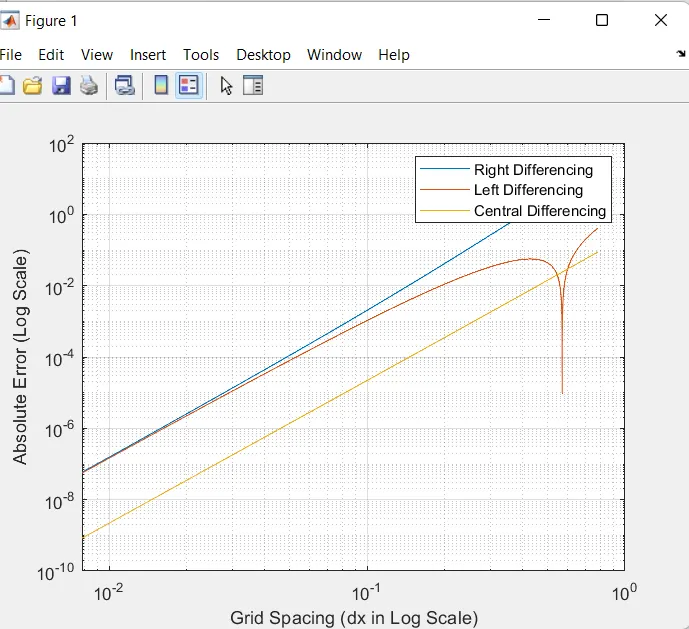

EXPLANATION:

1) first we are going to start a programe with clear all, close all,clc.

2) Then we are going to give Inputs of this function, then we need to use the linespace command of this stepsize range.

3) we need to calculate the analytical derivative of this function

4) then we have to calculate the skewed right sided (4th order approximation)and skwed left sided (4th order approximation)of the function.

5) And central differencing method(4th order approximation) then solving for the coefficients

6) then we need to write the anonymous function.

7) we have to calculate the numerical derivative with respect to right difference, left difference ,and central difference . and we calculate absolute error.

8) then we have to plot this function using the hold on command and grid ,x label ,y label ,legend command.

9) finally we got a plot for 4th order approximation of a 2nd order derivative .