Week 3 - External flow simulation over an Ahmed body.
Objective:- For this challenge, you will have to provide answers to the following questions:
Q1. Describe Ahmed's body and its importance.
Q2. Explain the reason for the negative pressure in the wake region.
Q3. Explain the significance of the point of separation.
Expected Results:
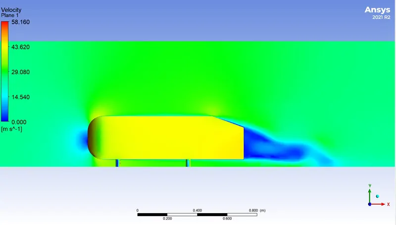
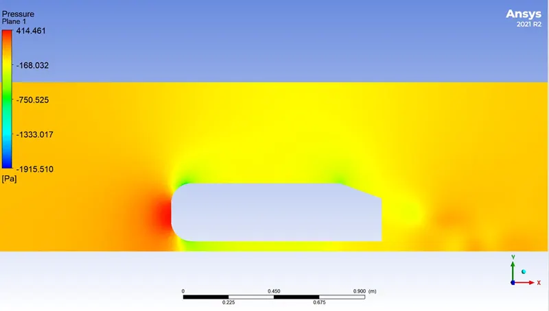
- Velocity and pressure contours.
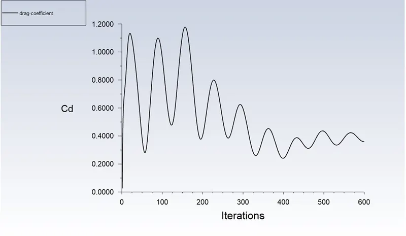
- The drag coefficient plot for a refined case. ( For velocity of 25m/sec, the drag coefficient should be around 0.33).
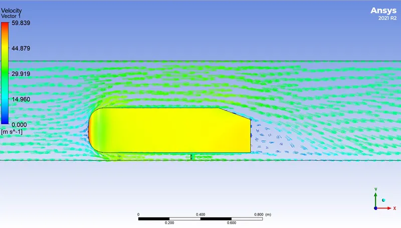
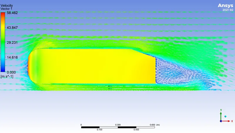
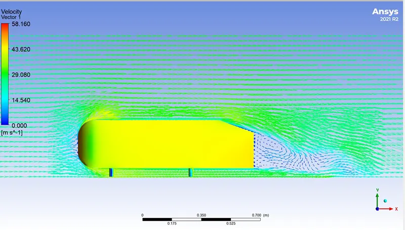
- The vector plot clearly showing the wake region.
- Perform the grid independency test and provide the values of drag and lift with each case.
Introduction:-
Ahmed Body and its Importance
The purpose of Ahmed Body is to provide a general reference with a lot of available experimental and numerical data to test the types of flows we do find in cars, i.e Vortices behind the car, straight body, ground interaction, and blunt nose. It is a good model to test a computational method or a general body modification prior to going-on with a more thorough analysis with an actual car geometry for which obtaining wind-tunnel data is costly and creating a mesh is a lengthy process.
People working in vehicle aerodynamics use Ahmed Body to validate their numerical model because the experimental data from wind tunnel testing is available for Ahmed Body. Once the numerical model is validated, it is used to design new models of the car.
Reason for Negative Pressure in the Wake region
When the air moving over the vehicle is separated at the rear end, it leaves a large low pressure turbulent region behind the vehicle known as the Wake. This wake contributes to the formation of pressure drag, which eventually reduces the vehicle performance.
Significance of point of separation
The position at which the boundary layer leaves the surface of a solid body is known a the separation point. It may occur with the laminar flow (laminar separation) or when the boundary layer is turbulent (turbulent separation). Separation is sometimes followed by reattachment of the flow. When an object is moving through any fluid medium, the fluid molecules push back on it and resist the object’s movement. This resistance is called Pressure Drag. As the fluid flows around the object, it sticks to the object, forming what is known as the boundary layer. This attached flow is flowing very smoothly. The point on the body where the boundary layer lifts off the surface is called the separation point. When the air flow separates off the surface, the pressure darg usually increases.
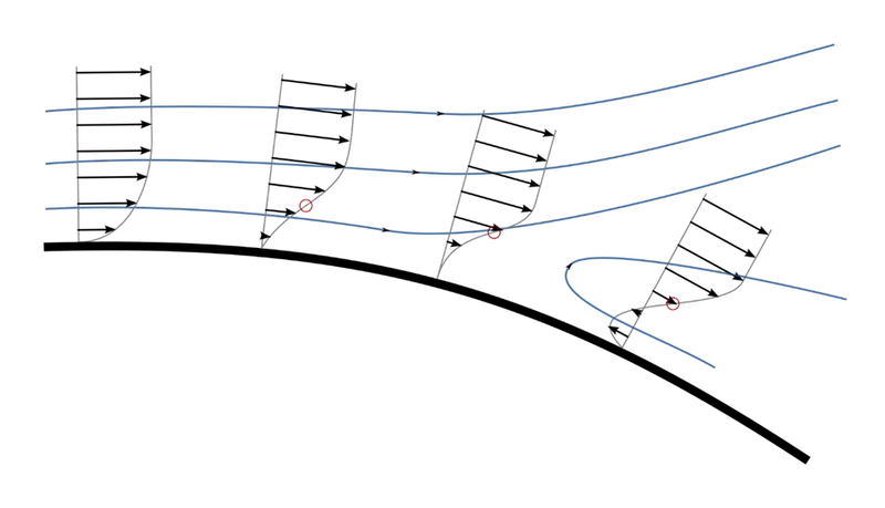
As the fluid passes over the surface, it is initially accelerating and so the pressure is decreasing in the direction of flow. This is called a Favourable Pressure Gradient (`(delp)/(delx)<0`). Beyond a certain point, the flow begins to Decelerate, and so the pressure in the direction of flow is increasing. This increase in pressure is called Adverse Pressure Gradient (`(delp)/(delx) >0`) and it has significant effect on the flow close to the wall. If the pressure increase is large enough, the flow will reverse its direction and since it cant travel backwards because of the incoming fluid, it detaches from the surface, resulting in flow separation
Procedure:-
Setting up of the model
Importing the model in spaceclaim
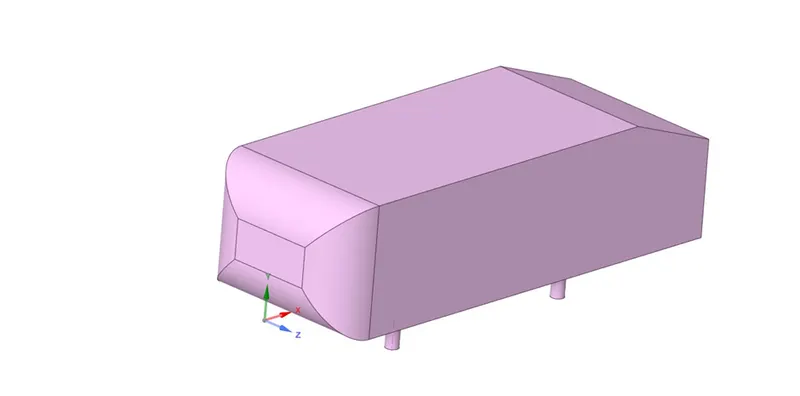
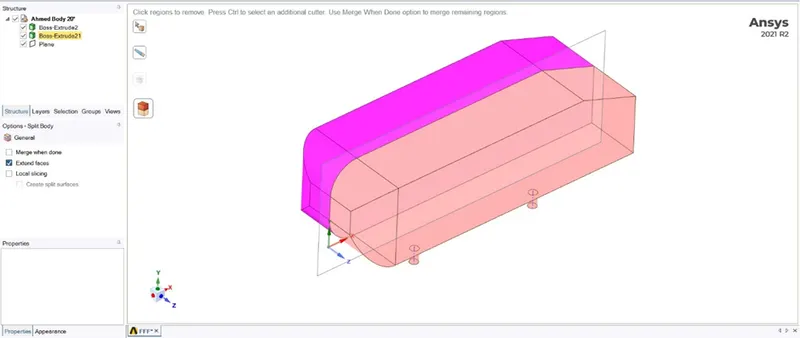
Since the model is symmetric, we will use the ‘split body’ command and run the simulation by considering only half the body. Here we can save on the number of cells and get the results faster as well.
Since the body is symmetric in X-Y plane, so we will first create the plane from ‘Design’ option as shown below.
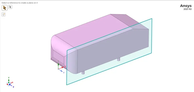
After this we will move the plane to the middle of the body in Z direction by using the ‘Move’ command
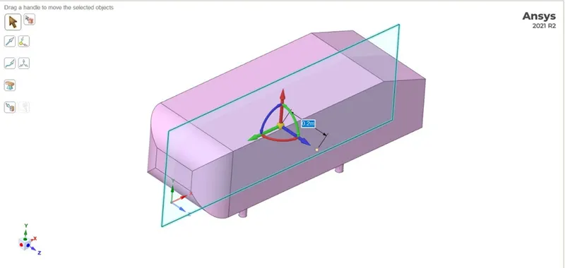
Now using the ‘Split Body’ command to split the given model in half.
Case 1:- Making an enclosure for the model (1 enclosure)
Meshing
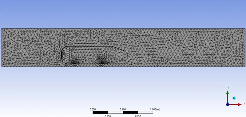
Here only one enclosure is used for meshing.
The element size used here is 0.05m
Also provide the boundary names
Pre-processing
Here we will use the density based solver in steady state simulation because mach number is greater than 0.3. In such conditions the Density-based solvers give a much accurate result as compared to the Pressure-based solvers.
Also the Reynolds number is high so the flow is turbulent. Hence we will use the k-epsilon turbulence model with standard wall function.
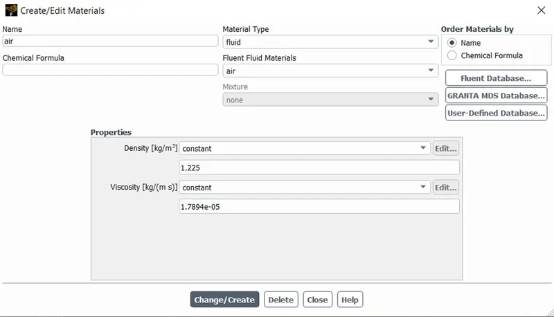
The fluid which is used in the simulation will be air
Setting up of the Physics
Boundary conditions
- Inlet – Velocity Inlet (25 m/s)
- Outlet – Pressure Outlet (0 pa)
- Car wall – No slip
- Symmetry
Also setting the reference values at the inlet for the calculation of the coefficient of Drag and Lift
The system is initialized using hybrid initialization and then run for 600 iterations.
Results
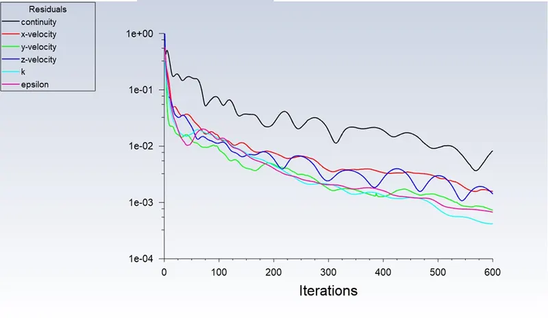
Residual plot
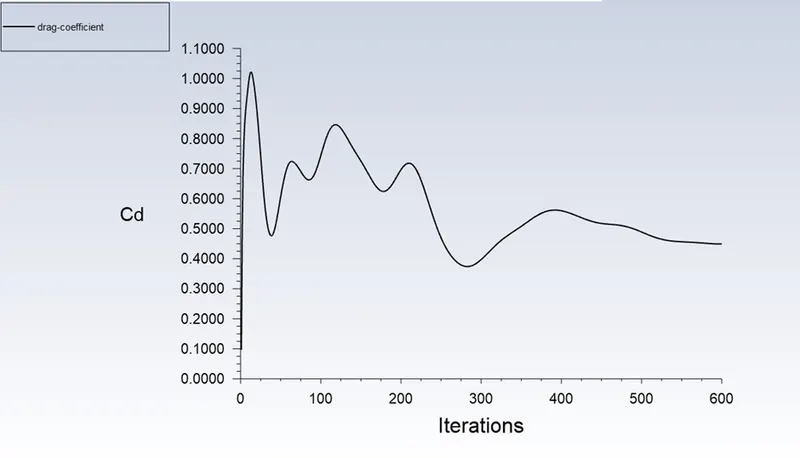
Coefficient of Darg
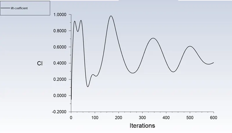
Coefficient of Lift
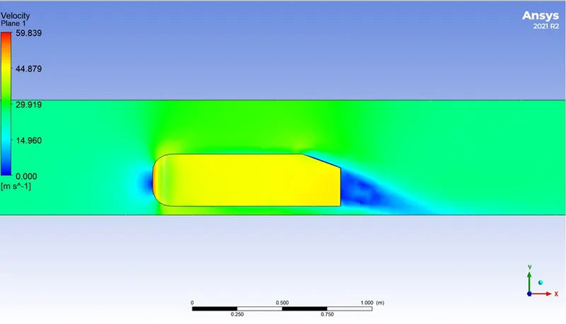
Velocity contour
Pressure contour
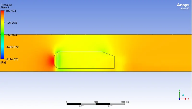
Vector representation of Velocity
Case 2:- Making an enclosure for the model (2 enclosure)
Meshing
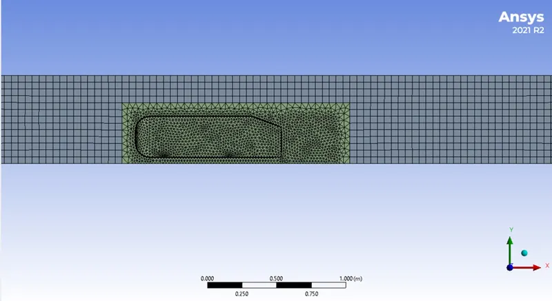
There are two encloser’s to be meshed. The outer one will be meshed with ‘Multizone’ method so that we get hexa mesh which has the highest quality of mesh. The inner enclosure will be meshed with ‘Tetrahedrons’ because almost all the phenomenon will be occurring in this part only.
The elements size used to mesh the first enclosure is 0.05m and the second enclosure is meshed with an element size of 0.02m
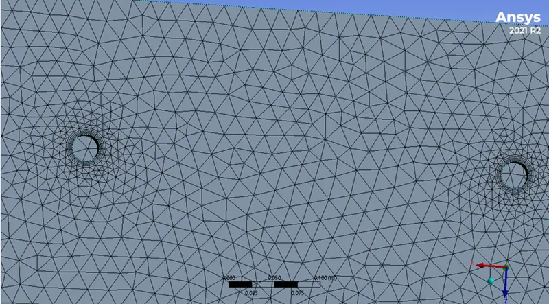
The cylinder which is below the car model will be approximated as some sort of polygon by fluent, so to resolve this we will insert a sizing method to this two cylinders.
Selecting the element size as 5mm and updating the mesh
Pre-processing
Here we will use the density based solver in steady state simulation because mach number is greater than 0.3. In such conditions the Density-based solvers give a much accurate result as compared to the Pressure-based solvers.
Also the Reynolds number is high so the flow is turbulent. Hence we will use the k-epsilon turbulence model with standard wall function.
The fluid which is used in the simulation will be air
Setting up of the Physics
Boundary conditions
- Inlet – Velocity Inlet (25 m/s)
- Outlet – Pressure Outlet (0 pa)
- Car wall – No slip
- Symmetry
Also setting the reference values at the inlet for the calculation of the coefficient of Drag and Lift
The system is initialized using hybrid initialization and then run for 600 iterations.
Results
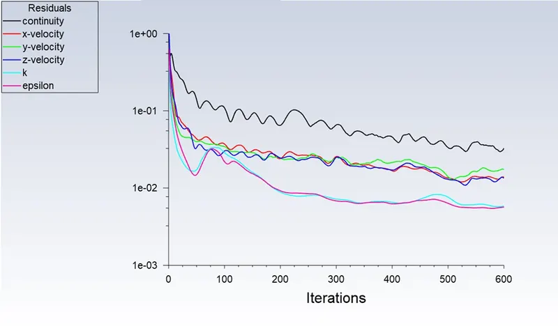
Residual plot
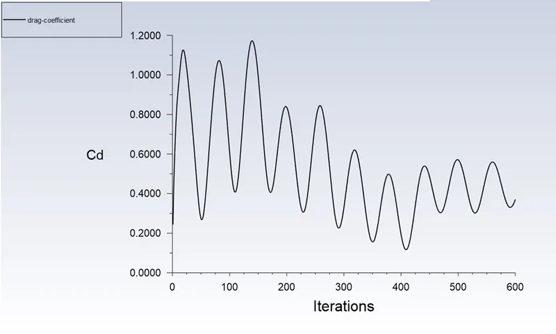
Coefficient of Drag
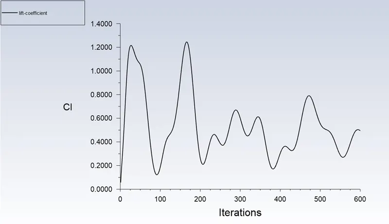
Coefficient of lift
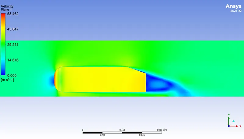
Velocity contour
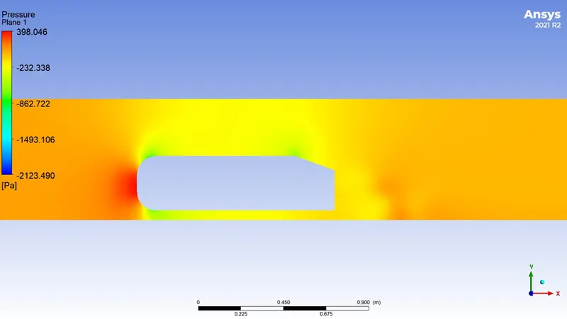
Pressure contour
Vector representation of Velocity
Case 3:- Making an enclosure for the model (2 enclosure with more finer mesh)
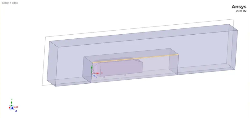
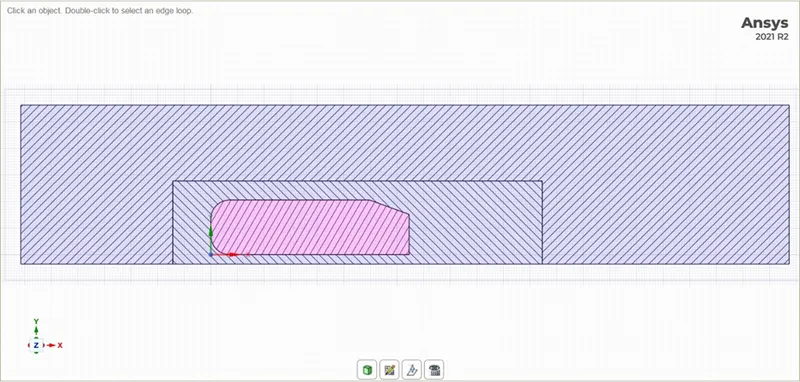
Checking and Resolving for any Interferences between both the enclosure and the model using the ‘Section Mode’
Meshing
There are two encloser’s to be meshed. The outer one will be meshed with ‘Multizone’ method so that we get hexa mesh which has the highest quality of mesh. The inner enclosure will be meshed with ‘Tetrahedrons’ because almost all the phenomenon will be occurring in this part only.
The elements size used to mesh the first enclosure is 0.04m and the second enclosure is meshed with an element size of 0.02m
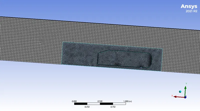
The cylinder which is below the car model will be approximated as some sort of polygon by fluent, so to resolve this we will insert a sizing method to this two cylinders.
Selecting the element size as 5mm and updating the mesh
It is very important phenomenon for refining a mesh because near the wall the centre of elements does not lie in a single lie and we don’t get the proper information near the walls. So here we will use the boundary layer phenomenon. By using the appropriate boundary layer thickness, we can create the boundary layer. First, calculate the first layer thickness using the y+ value for a given velocity, density, viscosity and length. We can select a value of y+ between 30-300 for k-epsilon with standard wall function turbulence model.
In this case to start with we will use y+ as 35
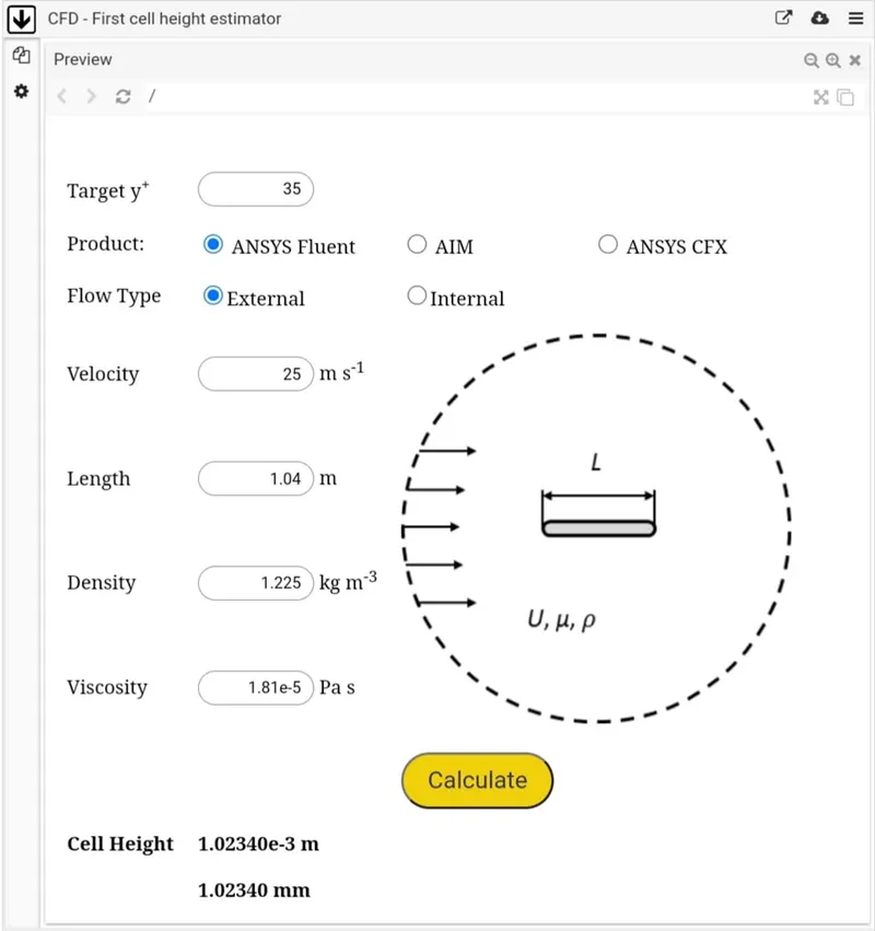
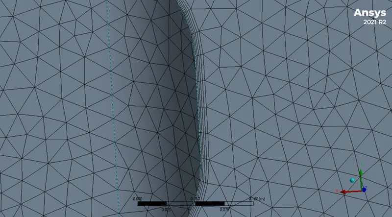
First layer thickness: 1.0234mm
No. of inflation layer: 5
Total thickness: 2.546546mm
Pre-processing
Here we will use the density based solver in steady state simulation because mach number is greater than 0.3. In such conditions the Density-based solvers give a much accurate result as compared to the Pressure-based solvers.
Also the Reynolds number is high so the flow is turbulent. Hence we will use the k-epsilon turbulence model with standard wall function.
The fluid which is used in the simulation will be air
Setting up of the Physics
Boundary conditions
- Inlet – Velocity Inlet (25 m/s)
- Outlet – Pressure Outlet (0 pa)
- Car wall – No slip
- Symmetry
Also setting the reference values at the inlet for the calculation of the coefficient of Drag and Lift
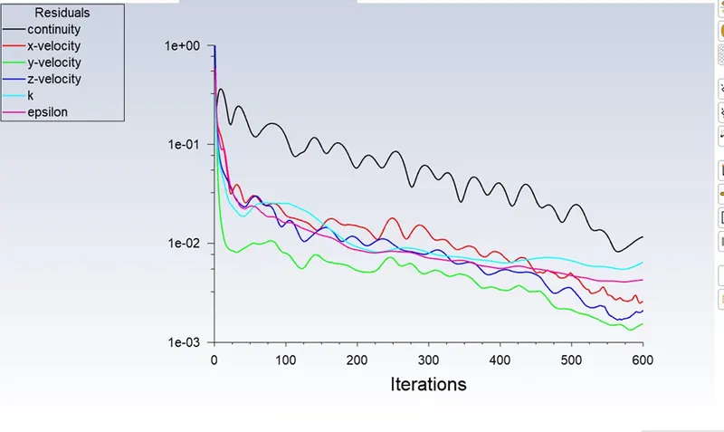
The system is initialized using hybrid initialization and then run for 600 iterations.
Results
Residual plot
Coefficient of Drag
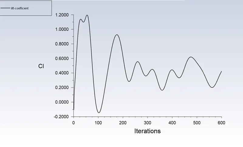
Coefficient of lift
Velocity contour
Pressure contour
Vector representation of Velocity
Results:-
|
Case 1 |
Case 2 |
Case 3 |
|
|
Coefficient of Drag |
0.449 |
0.36 |
0.3708 |
|
Coefficient of Lift |
0.408 |
0.424 |
0.4945 |
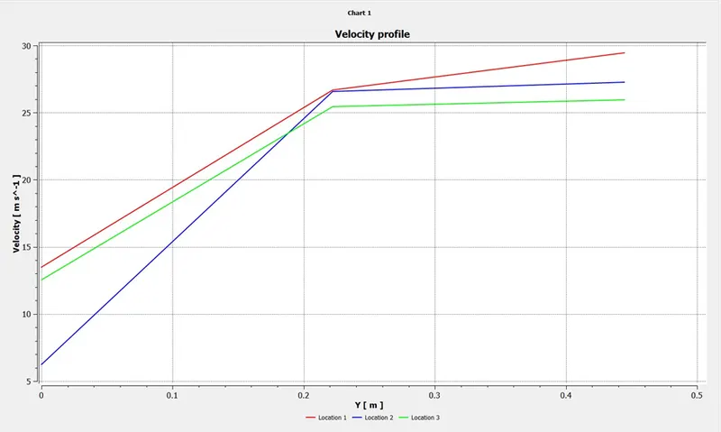
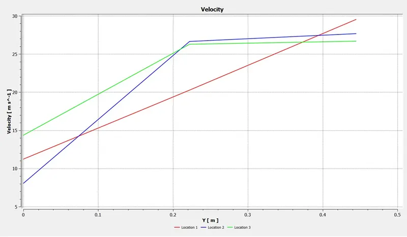
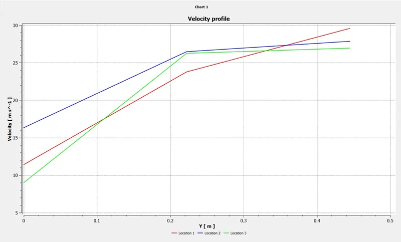
Velocity Plots for all the three cases at three different points
Case 1
Case 2
Case 3