Week 3 - Adiabatic Flame Temperature calculation

AIM: Exploration of Adiabatic Flame Temperature for different cases as mentioned below:

1. Adiabatic flame temperature variation with Equivalence ratio (In constant volume-chamber) :

2. Adiabatic flame temperature variation with Heat loss (In constant pressure-chamber) :

3. Adiabatic flame temperature variation with respect to Alkane, Alkene, Alkyne :

4. Adiabatic flame temperature variation with respect to a number of Carbon atom chains :

Introduction:

Adiabatic Flame Temperature is the temperature of combustion products, when thecombustion reaction energy is released to the combustion products, assuming no heat is lost in this process. There are to types of Adiabatic Flame Temperatures

1. Constant Volume Adiabatic Flame Temperature
2. Constant Pressure Adiabatic Flame Temperature

The constant volume adiabatic flame temperature is the temperature of combustion products from a complete combustion process that occurs without any work, heat transfer or changes in kinetic or potential energy. This temperature is higher than the constant pressure process because no energy is utilized to change the volume of the system.

Calculation of Adiabatic Flame Temperature can be done using Enthalpy difference method as well as Gibbs free energy minimization method. Gibbs free energy minimization method is considered to be more accurate, since calculation of enthalpy of all possible product formations and its mole fractions is difficult to achieve.

1. Adiabatic flame temperature variation with Equivalence ratio (In constant volume-chamber) :

Assume that methane is contained in a constant volume chamber. Write a program in Python to plot the effect of equivalence ratio on the final adiabatic flame temperature. Compare the results with Cantera. Assume that N2 is present. Upload your results as a picture and provide a link to your python program (google drive or Dropbox).

You need to paste the images in your answer box and explain the results.

The correct trend for the AFT vs equivalence ratio will only be obtainable if you use the Cantera module.

Ans:

For a constant voume combustion, equation to be solved:

In a constant volume process the internal energy of the products and reactants is constant, since work done is zero.

`U_(Reactants)*T*P=U_(Products)*T_(AFT)*P_(AF)`

Also

H=U+PV

PV=nRT

Solving above equations, we obtains

`H_(Reactants)-(nRT)_(reactants)=H_(Products)-(NRT)_(Products``

Hence, Equation to be solved: `(H_Products-H_Reactants)-R*(N_Products*T-N_Reactants*T_STP)=0`

Equivalence ratio : An ideal fuel/air mixture in which both the fuel and the oxygen in the air are completely consumed is called the stoichiometric mixture.If more air is supplied then the mixture is called a lean mixture and if less quantity of air is supplied then the mixture is called a rich mixture.

`phi=(A/F)_(st)/(A/F)`

For complete combustion: i. e stoichiometric mixture, phi=1

`C_xH_y+a(O_2+3.76N_2)=xCO_2+(y/2)H_2O+3.76aN_2`

The generalised equation :

`C_xH_y+a(O_2+3.76N_2)=xCO_2+(y/2)H_2O+3.76aN_2+bO_2+eCO`

For lean mixture: (More air)

`C_xH_y+a(O_2+3.76N_2)=xCO_2+(y/2)H_2O+3.76aN_2+bO_2`

For rich fuel mixture:

`C_xH_y+a(O_2+3.76N_2)=xCO_2+(y/2)H_2O+3.76aN_2+eCO`

#Adiabatic flame temperature variation with Equivalence ratio (In constant volume-chamber)
#Jayaram Oneil
#Methane combustion_Numerical
# Assuming constant volume system

import matplotlib.pyplot as plt
import math
import numpy as np
import cantera as ct
Tstp=298.15 # Temperature (K)
R = 8.314  # J/mol-K

def h(T, co_effs):  # Function to evaluate enthalpy
    a1 = co_effs[0]
    a2 = co_effs[1]
    a3 = co_effs[2]
    a4 = co_effs[3]
    a5 = co_effs[4]
    a6 = co_effs[5]

    return (a1*T + a2 * pow(T, 2) / 2 + a3 * pow(T, 3) / 3 + a4 * pow(T, 4) / 4 + a5 * pow(T, 5) / 5 + a6 ) * R


# reactants at STP ==> Low temp coeff
ch4_coeffs_l = [5.14987613E+00, -1.36709788E-02, 4.91800599E-05, -4.84743026E-08, 1.66693956E-11, -1.02466476E+04,
                -4.64130376E+00]
o2_coeffs_l = [3.78245636E+00, -2.99673416E-03, 9.84730201E-06, -9.68129509E-09, 3.24372837E-12, -1.06394356E+03,
               3.65767573E+00]
n2_coeffs_l = [0.03298677E+02, 0.14082404E-02, -0.03963222E-04, 0.05641515E-07, -0.02444854E-10, -0.10208999E+04,
               0.03950372E+02]

# products at unknown temp ==> high temp coeff
n2_coeffs_h = [0.02926640E+02, 0.14879768E-02, -0.05684760E-05, 0.10097038E-09, -0.06753351E-13, -0.09227977E+04,
               0.05980528E+02]
co2_coeffs_h = [3.85746029E+00, 4.41437026E-03, -2.21481404E-06, 5.23490188E-10, -4.72084164E-14, -4.87591660E+04,
                2.27163806E+00]
h2o_coeffs_h = [3.03399249E+00, 2.17691804E-03, -1.64072518E-07, -9.70419870E-11, 1.68200992E-14, -3.00042971E+04,
                4.96677010E+00]
co_coeffs_h = [2.71518561E+00, 2.06252743E-03, -9.98825771E-07, 2.30053008E-10, -2.03647716E-14, -1.41518724E+04, 7.81868772E+00]
o2_coeffs_h = [3.28253784E+00, 1.48308754E-03, -7.57966669E-07, 2.09470555E-10, -2.16717794E-14, -1.08845772E+03, 5.45323129E+00]



def f(T, phi):
    h_ch4_r = h(Tstp, ch4_coeffs_l)
    h_o2_r = h(Tstp, o2_coeffs_l)
    h_n2_r = h(Tstp, n2_coeffs_l)

    H_reactants = h_ch4_r + (2 / phi) * h_o2_r + (7.52 / phi) * h_n2_r
    dPV_reactants = (1 + (2 / phi) + (7.52 / phi)) * R * Tstp

    h_co2_p = h(T, co2_coeffs_h)
    h_h2o_p = h(T, h2o_coeffs_h)
    h_n2_p = h(T, n2_coeffs_h)
    h_co_p = h(T, co_coeffs_h)
    h_o2_p = h(T, o2_coeffs_h)

    if phi >= 1:
        H_products = (4 / phi - 3) * h_co2_p + 2 * h_h2o_p + (7.52 / phi) * h_n2_p + (4 - 4 / phi) * h_co_p
        dPV_products = ((4 / phi - 3) + 2 + (7.52 / phi) + (4 - 4 / phi)) * R * T

    elif phi < 1:
        H_products = h_co2_p + 2 * h_h2o_p + (7.52 / phi) * h_n2_p + (2 / phi - 2) * h_o2_p
        dPV_products = (1 + 2 + (7.52 / phi) + (2 / phi - 2)) * R * T

    return (H_products - H_reactants) - (dPV_products - dPV_reactants)


# Defining the derivative of function
def fprime(T, phi):
    return (f(T + 1e-6, phi) - f(T, phi)) / (1e-6)


# Newton-Raphson
alpha = 0.9
tol = 1e-3
phi = np.arange(0.1,2.1,0.1)

T_AFT = []

for i in range(0, len(phi)):
    T_guess = 1500  # K
    while abs(f(T_guess, phi[i])) >= tol:
        T_guess = T_guess - alpha * ((f(T_guess, phi[i])) / (fprime(T_guess, phi[i])))
    T_AFT.append(T_guess)

print(T_AFT)
print()

#cantera
gas = ct.Solution('gri30.xml')
T_AFT_ct = []

# Computing mole fractions
for i in range(0,len(phi)):
    n_total= 1 + (2/phi[i]) + (7.52/phi[i])
    n_ch4 = 1/n_total
    n_o2 = (2/phi[i])/n_total
    n_n2 = (7.52/phi[i])/n_total
# Defining the gas mixture
    gas.TPX = 298.15, 101325, {'CH4':n_ch4, 'O2':n_o2, 'N2':n_n2}
# Calculating the equilibrium conditions
    gas.equilibrate('UV','auto')
    T_AFT_ct.append(gas.T)

print(T_AFT_ct)

# Plotting
plt.plot(phi,T_AFT,'-x',color='red',label='Python')
plt.plot(phi, T_AFT_ct, '-o',color='blue',label='Cantera')
plt.xlabel('Equivalence Ratio ($phi$)', fontsize=12)
plt.ylabel('Adiabatic Flame Temperature [K]', fontsize=12)
plt.yticks(np.arange(600, 3100, step=200))
plt.xticks(np.arange(0, 2.2, step=0.2))
plt.grid('on')
plt.title('Adibatic Flame Temperature vs. Equivalence Ratio \n Methane-Air Combustion', fontsize=10, fontweight='bold')
plt.legend(fontsize=10)
plt.show()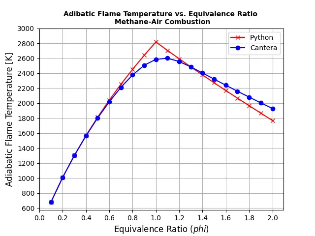

Value Comparison: Python Vs Cantera

Phi	Python	Cantera
0.1	681.684584	679.6185876
0.2	1009.55283	1009.439689
0.3	1301.87037	1300.749034
0.4	1567.8622	1563.55559
0.5	1812.87595	1802.08879
0.6	2040.41614	2018.372584
0.7	2252.98108	2211.713985
0.8	2452.45989	2377.513793
0.9	2640.34098	2506.672869
1	2817.83102	2585.878267
1.1	2704.16713	2600.539167
1.2	2592.95404	2556.491324
1.3	2484.00521	2484.065137
1.4	2377.13279	2403.256251
1.5	2272.14744	2321.028551
1.6	2168.85803	2239.550449
1.7	2067.07139	2159.515353
1.8	1966.59179	2081.141912
1.9	1867.22023	2004.483953
2	1768.75343	1929.532724

Major observation:

1. Temperature observed by python is higher, since complete products of combustion has not been considered in the python approach.
2. Highest temperature observed near stoichiometric composition in both python code as well as using cantera.
3. Cantera provide a continous curve.
4. Adiabatic Flame temperature is continously rising upto or nearby stoichiometric composition and reduces with further increase in Equivalence ratio.

2. Adiabatic flame temperature variation with Heat loss (In constant pressure-chamber) :

Consider a constant pressure reactor with heat loss. The reactor is initially set at STP conditions.

The heat loss should be input in your program and must be a fraction of the "maximum possible heat loss". You will control heat loss using a variable called H_loss. For example, H_loss = 0.5 would mean a heat loss that is equal to 50% of the maximum possible heat loss.

The fuel type can be a general hydrocarbon of the form CxHy. Phi and lambda = 1.0. Find the AFT of CH4 with H_loss = 0.35

Ans:

For a constant pressure combustion, enthaly difference is the equation to be solved:

`(H_Products-H_Reactants)=0`

Considering Heat loss, equation is modified as :

`(H_Products-H_Reactants)-(Heat Loss Coefficient*(H_Products-H_Reactants)) =0`

#Adiabatic flame temperature with heat loss (In constant pressure-chamber)
#Jayaram Oneil
#Methane combustion_Numerical
# Assuming constant pressure system


import matplotlib.pyplot as plt
import math
import numpy as np
import cantera as ct
Tstp=298.15 # Temperature (K)
R = 8.314  # J/mol-K

def h(T, co_effs):  # Function to evaluate enthalpy
    a1 = co_effs[0]
    a2 = co_effs[1]
    a3 = co_effs[2]
    a4 = co_effs[3]
    a5 = co_effs[4]
    a6 = co_effs[5]

    return (a1*T + a2 * pow(T, 2) / 2 + a3 * pow(T, 3) / 3 + a4 * pow(T, 4) / 4 + a5 * pow(T, 5) / 5 + a6 ) * R


# reactants at STP ==> Low temp coeff
ch4_coeffs_l = [5.14987613E+00, -1.36709788E-02, 4.91800599E-05, -4.84743026E-08, 1.66693956E-11, -1.02466476E+04,
                -4.64130376E+00]
o2_coeffs_l = [3.78245636E+00, -2.99673416E-03, 9.84730201E-06, -9.68129509E-09, 3.24372837E-12, -1.06394356E+03,
               3.65767573E+00]
n2_coeffs_l = [0.03298677E+02, 0.14082404E-02, -0.03963222E-04, 0.05641515E-07, -0.02444854E-10, -0.10208999E+04,
               0.03950372E+02]

# products at unknown temp ==> high temp coeff
n2_coeffs_h = [0.02926640E+02, 0.14879768E-02, -0.05684760E-05, 0.10097038E-09, -0.06753351E-13, -0.09227977E+04,
               0.05980528E+02]
co2_coeffs_h = [3.85746029E+00, 4.41437026E-03, -2.21481404E-06, 5.23490188E-10, -4.72084164E-14, -4.87591660E+04,
                2.27163806E+00]
h2o_coeffs_h = [3.03399249E+00, 2.17691804E-03, -1.64072518E-07, -9.70419870E-11, 1.68200992E-14, -3.00042971E+04,
                4.96677010E+00]

Max_heat_loss=h(Tstp,ch4_coeffs_l) + 2*h(Tstp,o2_coeffs_l) - h(Tstp,co2_coeffs_h) - 2*h(Tstp,h2o_coeffs_h)

def f(T, H_losscoeff):
    # enthalpy of products
    h_co2_p = h(T, co2_coeffs_h)
    h_h2o_p = h(T, h2o_coeffs_h)
    h_n2_p = h(T, n2_coeffs_h)
    H_products= h_co2_p + 2 * h_h2o_p + 7.52 * h_n2_p

    # enthalpy of reactants

    h_ch4_r = h(Tstp, ch4_coeffs_l)
    h_o2_r = h(Tstp, o2_coeffs_l)
    h_n2_r = h(Tstp, n2_coeffs_l)
    H_reactants= h_ch4_r + 2 * h_o2_r + 7.52 * h_n2_r

    dH = H_reactants - H_products
    return dH - (H_losscoeff * Max_heat_loss)



def fprime(T,H_losscoeff):
    return (f(T + 1e-6, H_losscoeff) - f(T, H_losscoeff)) / 1e-6


H_losscoeff = 0
T_AFT = []
H_loss = []


while (H_losscoeff < 1):
    # Newton raphson technique
    tol = 1e-4
    alpha = 0.1
    ct = 0
    T_guess = 1500
    while (abs(f(T_guess, H_losscoeff)) > tol):
        T_guess = T_guess - alpha * ((f(T_guess, H_losscoeff) / fprime(T_guess,H_losscoeff)))
        ct = ct + 1
    print(T_guess,ct)
    H_loss.append(H_losscoeff)
    T_AFT.append(T_guess)
    H_losscoeff = H_losscoeff + 0.1

H_losscoeff = 0.35
while (abs(f(T_guess, H_losscoeff)) > tol):
    T_guess = T_guess - alpha * ((f(T_guess, H_losscoeff) / fprime(T_guess, H_losscoeff)))
print(T_guess)
T_guess_calc=T_guess
plt.plot(0.35,T_guess,'-o',color='blue')

# Plotting
plt.plot(H_loss,T_AFT,'-x',color='red',label='Python')
plt.title('Adibatic Flame Temperature vs. Heat Loss \n Phi=1', fontsize=10, fontweight='bold')
plt.yticks(np.arange(100, 3100, step=200))
plt.xticks(np.arange(0, 1.2, step=0.2))
plt.xlabel('Heat Loss coeff ', fontsize=12)
plt.ylabel('Adiabatic Flame Temperature [K]', fontsize=12)
plt.grid('on')
plt.legend(fontsize=10)
plt.show()

For Heat Loss coeff of 03.35, Adiabatic Flame Temperature=1678.805K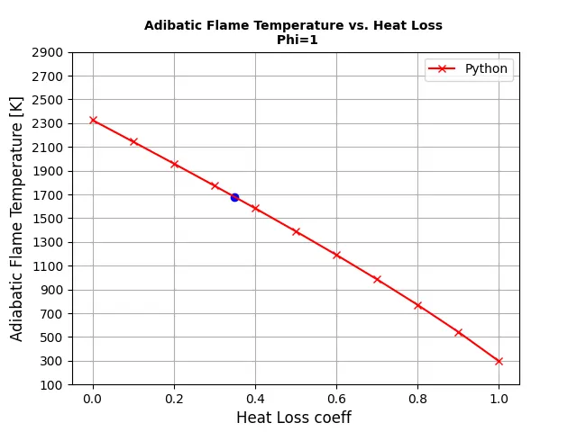

Heat Loss coefficient	Adiabatic Flame Temperature (K)
0	2325.5981295353686 209
0.1	2143.6727828882913 207
0.2	1959.709224280915 204
0.3	1773.2060879269486 199
0.4	1583.5096887744405 187
0.5	1389.7572758813405 190
0.6	1190.7871515371999 199
0.7	984.9884135301207 204
0.8	770.0321538475063 207
0.9	542.3457434347945 210
1	295.9482117282339 212

Major Observations:

1. Adiabatic flame temperature decreases as heat loss increases.
2. AFT when Heat loss is minimum, is 2325.6K and when Heat Loss is maximum is 295.94 K

3. Adiabatic flame temperature variation with respect to Alkane, Alkene, Alkyne :

Test it only for Alk-ane, -ene and -yne variants of 2 Carbon atom chain and plot a trend. The provided therm.dat might not contain data for other alkanes, alkynes, and alkenes (in that case use Cantera). Assume no heat loss.

Ans:

Considering stioichiometric mixture with no heat lose and at constant pressure

Ethane: `C_2H_6 + 3.5(O_2 + 3.76N_2) <=> 2CO_2 + 3H_2O + 13.16N_2`

Ethene: `C_2H_4 + 3(O_2 + 3.76N_2) <=> 2CO_2 + 2H_2O + 11.28N_2`

Ethyne: `C_2H_2 + 2.5(O_2 + 3.76N_2) <=> 2CO_2 + H_2O + 9.4N_2`

#Adiabatic flame temperature variation with respect to Alkane, Alkene, Alkyne :
#Jayaram Oneil
# Assuming constant pressure system


import matplotlib.pyplot as plt
import math
import numpy as np
import cantera as ct
Tstp=298.15 # Temperature (K)
R = 8.314  # J/mol-K
# Function to calculate enthalpy of a compound through NASA polynomial function
def h(T, coeff):
	a1 = coeff[0]
	a2 = coeff[1]
	a3 = coeff[2]
	a4 = coeff[3]
	a5 = coeff[4]
	a6 = coeff[5]
	return (a1 + a2*T/2 + a3*pow(T,2)/3 + a4*pow(T,3)/4 + a5*pow(T,4)/5 + a6/T)*R*T

# Coefficients for low temperatures
c2h6_coeffs_l = [4.29142492E+00, -5.50154270E-03, 5.99438288E-05, -7.08466285E-08, 2.68685771E-11, -1.15222055E+04, 2.66682316E+00]
c2h4_coeffs_l = [3.95920148E+00, -7.57052247E-03, 5.70990292E-05, -6.91588753E-08, 2.69884373E-11, 5.08977593E+03, 4.09733096E+00]
c2h2_coeffs_l = [8.08681094E-01, 2.33615629E-02, -3.55171815E-05, 2.80152437E-08, -8.50072974E-12, 2.64289807E+04, 1.39397051E+01]
o2_coeffs_l = [3.78245636E+00, -2.99673416E-03, 9.84730201E-06, -9.68129509E-09, 3.24372837E-12, -1.06394356E+03, 3.65767573E+00]
n2_coeffs_l = [0.03298677E+02, 0.14082404E-02, -0.03963222E-04, 0.05641515E-07, -0.02444854E-10, -0.10208999E+04, 0.03950372E+02]

# Coefficients for high temperatures
co2_coeffs_h = [3.85746029E+00, 4.41437026E-03, -2.21481404E-06, 5.23490188E-10, -4.72084164E-14, -4.87591660E+04, 2.27163806E+00]
h2o_coeffs_h = [3.03399249E+00, 2.17691804E-03, -1.64072518E-07, -9.70419870E-11, 1.68200992E-14, -3.00042971E+04, 4.96677010E+00]
n2_coeffs_h = [0.02926640E+02, 0.14879768E-02, -0.05684760E-05, 0.10097038E-09, -0.06753351E-13, -0.09227977E+04, 0.05980528E+02]
# Standard temperature condition
Tstp = 298.15 # K

# Defining the function for root-solving by Newton-Raphson method
def f(T, ncarbon):
    h_c2h6_r = h(Tstp, c2h6_coeffs_l)
    h_c2h4_r = h(Tstp, c2h4_coeffs_l)
    h_c2h2_r = h(Tstp, c2h2_coeffs_l)
    h_o2_r = h(Tstp, o2_coeffs_l)
    h_n2_r = h(Tstp, n2_coeffs_l)
    h_co2_p = h(T, co2_coeffs_h)
    h_h2o_p = h(T, h2o_coeffs_h)
    h_n2_p = h(T, n2_coeffs_h)
    if ncarbon==1:
        x = 2
        y = 6
        h_fuel = h_c2h6_r
    elif ncarbon==2:
        x = 2
        y = 4
        h_fuel = h_c2h4_r
    elif ncarbon==3:
        x = 2
        y = 2
        h_fuel = h_c2h2_r
    H_reactants = h_fuel + (x+y/4)*h_o2_r + 3.76*(x+y/4)*h_n2_r
    H_products = x*h_co2_p + (y/2)*h_h2o_p + 3.76*(x+y/4)*h_n2_p
    return H_products - H_reactants

# Defining the derivative of the function
def fprime(T, ncarbon):
    return (f(T+1e-6, ncarbon) - f(T, ncarbon))/(1e-6)

# Newton-Raphson solver
alpha = 1
tol = 1e-3
ncarbon = [1, 2, 3]
T_AFT = []
for i in range(0,len(ncarbon)):
    T_guess = 1500 # K
    while abs(f(T_guess, ncarbon[i])) >= tol:
        T_guess = T_guess - alpha*((f(T_guess, ncarbon[i]))/(fprime(T_guess, ncarbon[i])))
    T_AFT.append(T_guess)
print(T_AFT)


# Plotting the Python results
plt.bar(['Ethane ($C_2H_6$)','Ethene ($C_2H_4$)','Ethyne ($C_2H_2$)'],T_AFT)
plt.ylabel('Adiabatic Flame Temperature (K)',fontsize=12)
plt.title('Adiabatic Flame Temperature  vs. Type of Hydrocarbon (Python)',fontsize=13,fontweight='bold')
plt.yticks(np.arange(100, 3100, step=200))
plt.xticks(np.arange(0, 3, step=1))
plt.grid('on')
plt.show()

#using cantera

gas = ct.Solution('gri30.xml')
T_AFT_ct = []
ncarbon = [1, 2, 3]
for i in range(0,len(ncarbon)):
        # Computing the mole fractions of each reactant
            if ncarbon[i]==1:
                x = 2
                y = 6
                fuel = 'C2H6'
            elif ncarbon[i]==2:
                x = 2
                y = 4
                fuel = 'C2H4'
            elif ncarbon[i]==3:
                x = 2
                y = 2
                fuel = 'C2H2'
            n_total = 1 + (x+y/4) + 3.76*(x+y/4)
            n_fuel = 1/n_total
            n_o2 = (x+y/4)/n_total
            n_n2 = (3.76*(x+y/4))/n_total
            gas.TPX = 298.15, 101325, {fuel: n_fuel, 'O2': n_o2, 'N2': n_n2}
            gas.equilibrate('HP', 'auto')
            T_AFT_ct.append(gas.T)
print(T_AFT_ct)

# Plotting Cantera results
plt.bar(['Ethane ($C_2H_6$)','Ethene ($C_2H_4$)','Ethyne ($C_2H_2$)'],T_AFT_ct)
plt.ylabel('Adiabatic Flame Temperature (K)',fontsize=12)
plt.title('AFT vs. Type of Hydrocarbon (Cantera)',fontsize=13,fontweight='bold')
plt.yticks(np.arange(100, 3100, step=200))
plt.xticks(np.arange(0, 3, step=1))
plt.grid('on')
plt.show()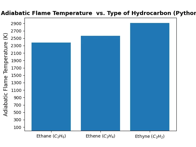

Major observations

1. It is observed from the Adiabatic Flame Temperature, that more energy is release when combustion of triple bond ethyne, compared to lesser bond hydrocarbon of same number of carbon atoms.

4. Adiabatic flame temperature variation with respect to a number of Carbon atom chains :

For a general alkane, plot the effect of the number of carbon atoms (from 1 to 3) on the final temperature. Assume no heat loss.

Ans:

Considering stioichiometric mixture with no heat lose and at constant pressure

Methane: `CH_4+2(O_2+3.76N_2 )→CO_2+2H_2 O+7.52N_2`

Ethane :`C_2 H_(6 )+3.5(O_2+3.76N_2 )→2CO_2+3H_2 O+13.16N_2`

Propane:`C_3 H_(8 )+5(O_2+3.76N_2 )→3CO_2+4H_2 O+18.8N_2`

#Adiabatic flame temperature variation with respect to a number of Carbon atom chains :
#Jayaram Oneil
#Assuming constant pressure system with no heat loss

#using cantera
import matplotlib.pyplot as plt
import math
import numpy as np
import cantera as ct
Tstp=298.15 # Temperature (K)
R = 8.314  # J/mol-K

gas = ct.Solution('gri30.xml')
T_AFT_ct = []
ncarbon = [1, 2, 3]
for i in range(0,len(ncarbon)):
        # Computing the mole fractions of each reactant
            if ncarbon[i]==1:
                x = 1
                y = 4
                fuel = 'CH4'
            elif ncarbon[i]==2:
                x = 2
                y = 6
                fuel = 'C2H6'
            elif ncarbon[i]==3:
                x = 3
                y = 8
                fuel = 'C3H8'
            n_total = 1 + (x+y/4) + 3.76*(x+y/4)
            n_fuel = 1/n_total
            n_o2 = (x+y/4)/n_total
            n_n2 = (3.76*(x+y/4))/n_total
            gas.TPX = 298.15, 101325, {fuel: n_fuel, 'O2': n_o2, 'N2': n_n2}
            gas.equilibrate('HP', 'auto')
            T_AFT_ct.append(gas.T)
print(T_AFT_ct)

# Plotting Cantera results
plt.bar(['Methane ($CH_4$)','Ethane ($C_2H_6$)','Propane ($C_3H_8$)'],T_AFT_ct)
plt.ylabel('Adiabatic Flame Temperature (K)',fontsize=12)
plt.title('AFT vs. Type of Hydrocarbon (Cantera)',fontsize=13,fontweight='bold')
plt.yticks(np.arange(100, 3100, step=200))
plt.xticks(np.arange(0, 3, step=1))
plt.grid('on')
plt.show()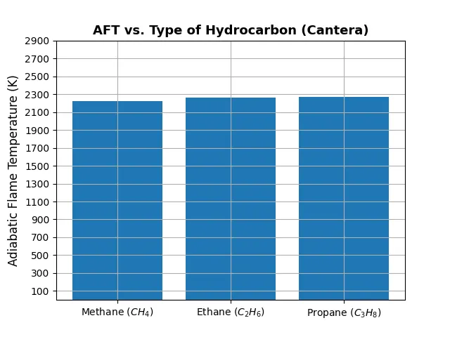

Major observations

1. Alkanes with carbon atoms of 1 to 3 have a adiabatic flame temperature difference of less than 50 K.
2. This lower difference may be attributed to simpler reaction of alkanes, compared to alkenes and alkynes.