Study of Adiabatic Flame Temperature using PYTHON and CANTERA
OBJECTIVES:
- To study the effect of equivalence ratio on the final Adiabatic Flame Temperature (in a Constant Volume chamber) and compare the results with Cantera.
- To study the Adiabatic Flame Temperature variation with heat loss in a Constant Pressure chamber.
- To calculate the Adiabatic Flame Temperature for different fuel types such as alkane, alkene, and alkynes.
- To calculate the Adiabatic Flame Temperature by varying the number of carbon atoms.
INTRODUCTION:
Combustion is a chemical process in which the fuel (solid, liquid, or gas) reacts rapidly with an oxidizer to release huge amounts of energy. During these reactions, energy is released to the combustion products and this energy in the form of heat increases the temperature of the combustion products inside the combustion chamber. The temperature rise depends upon the air-fuel ratio e.g. when we use an excess of oxidizer, the flame temperature is reduced.
- ADIABATIC FLAME TEMPERATURE: For a combustion process that takes place adiabatically with no shaft work, the temperature of the products is referred to as the adiabatic flame temperature. This is the maximum temperature that can be achieved for given reactants after the fuel is completely burned. It is an ideal case temperature and the actual flame temperature observed for a particular fuel is always less than this. Heat transfer, incomplete combustion, and dissociation all result in lower temperatures. The maximum adiabatic flame temperature for a given fuel and oxidizer combination occurs with a stoichiometric mixture (correct proportions such that all fuel and all oxidizers are consumed). The amount of excess air can be tailored as part of the design to control the adiabatic flame temperature.
- EQUIVALENCE RATIO, phi: It is defined as the ratio of the actual fuel-air ratio in the mixture to the stoichiometric fuel-air ratio. If the equivalence ratio is equal to one, the combustion is stoichiometric. If it is less than 1, the combustion is lean with excess air, and if it is greater than 1, the combustion is rich with incomplete combustion.
For Lean mixture (phi<1) -

For rich mixture (phi>1) -

- NEWTON RAPHSON: The Newton Raphson method is an iterative method to find the root of a function starting at a guess value and iterating till the value of the function f(x) reaches below a tolerance as-
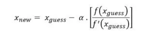
where α is the relaxation factor that determines the intensity of the iteration solver. For α < 1, the solution is under-relaxed and may take a greater number of iterations, which is called undershooting. For
α > 1, the solution overshoots and may lead to divergence.
- ENTHAPLY OF THE SYSTEM: The enthalpy of the reactants and products at a particular temperature is calculated using the NASA polynomial function-

where a1, a2, a3, a4, a5 and a6 are the coefficients from the thermodynamic data file - ''http://combustion.berkeley.edu/gri-mech/version30/files30/thermo30.dat''
Case 1: VARIATION OF ADIABATIC FLAME TEMPERATURE WITH THE EQUIVALENCE RATIO AT CONSTANT VOLUME
The first law of thermodynamics states that energy can be converted from one form to another with the interaction of heat, work and internal energy, but it can cannot be created or destroyed, under any circumstances. It is represented as-
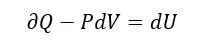
The constant volume adiabatic flame temperature is the temperature that results from a complete combustion process and occurs without any work, heat transfer, or changes in kinetic or potential energy. This temperature is higher than the constant pressure process because no energy is utilized to change the volume of the system. This is the maximum temperature that can be achieved because any heat transfer from the reacting substances or any incomplete combustion would tend to lower the temperature of the products.
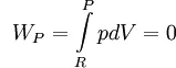
δQ = 0, as the process is adiabatic.
Therefore,
dU = 0
UR = UP
We know, H = U + PV, and PV = NRT therefore, the required equation is -
HR – HP – R*(NR*TSTP – NP*T) = 0
Code:
"""
AFT of Methane at different equivalence ratios

CH4 + 2(O2 + 3.76N2) = CO2 + 2H2O + 7.52N2

General Equation:

CxHy + g(O2 + 3.76N2) = a.CO2 + b.H2O + c.N2 + d.O2 + e.CO

"""

import matplotlib.pyplot as plt
import math
import numpy as np
import cantera as ct

# The equivalence ratio 'phi' is varied from 0.5 to 1.5

phi = np.linspace(0.5,1.5,101)

# Function to calculate the enthalpy using NASA polynomial function

def h(T, co_effs):

	R = 8.314 #J/mol-K
	a1 = co_effs[0]
	a2 = co_effs[1]
	a3 = co_effs[2]
	a4 = co_effs[3]
	a5 = co_effs[4]
	a6 = co_effs[5]

	return(a1 + a2*T/2 + a3*pow(T,2)/3 + a4*pow(T,3)/4 + a5*pow(T,4)/5 +a6/T)*R*T

# Low temp coefficients (reactants) at STP conditions

CH4_coeffs_l = [5.14987613E+00, -1.36709788E-02, 4.91800599E-05, -4.84743026E-08, 1.66693956E-11, -1.02466476E+04, -4.64130376E+00]

O2_coeffs_l = [3.78245636E+00, -2.99673416E-03, 9.84730201E-06, -9.68129509E-09, 3.24372837E-12, -1.06394356E+03, 3.65767573E+00]

N2_coeffs_l = [0.03298677E+02, 0.14082404E-02, -0.03963222E-04, 0.05641515E-07, -0.02444854E-10, -0.10208999E+04, 0.03950372E+02]

# High temp coefficients (products)

N2_coeffs_h = [0.02926640E+02, 0.14879768E-02, -0.05684760E-05, 0.10097038E-09, -0.06753351E-13, -0.09227977E+04, 0.05980528E+02]

CO2_coeffs_h = [3.85746029E+00, 4.41437026E-03, -2.21481404E-06, 5.23490188E-10, -4.72084164E-14, -4.87591660E+04, 2.27163806E+00]

H20_coeffs_h = [3.03399249E+00, 2.17691804E-03, -1.64072518E-07, -9.70419870E-11, 1.68200992E-14, -3.00042971E+04, 4.96677010E+00]

O2_coeffs_h = [3.28253784E+00, 1.48308754E-03, -7.57966669E-07, 2.09470555E-10, -2.16717794E-14, -1.08845772E+03, 5.45323129E+00]

CO_effs_h = [2.71518561E+00, 2.06252743E-03, -9.98825771E-07, 2.30053008E-10, -2.03647716E-14, -1.41518724E+04, 7.81868772E+00]

# Function for root-solving using NR method iteratively

def f(T, phi):

	R = 8.314
	x = 1
	y = 4

	if phi<=1:

		h_CO2_p = h(T,CO2_coeffs_h)
		h_N2_p = h(T,N2_coeffs_h)
		h_H2O_p = h(T,H20_coeffs_h)
		h_O2_p = h(T,O2_coeffs_h)

		H_products = h_CO2_p + 2*h_H2O_p + ((2/phi)-2)*h_O2_p + (7.52/phi)*h_N2_p
		N_products =  1 + 2 + ((2/phi) - 2) + (7.52/phi)

		Tstp = 298.15
		h_CH4_r = h(Tstp,CH4_coeffs_l)
		h_O2_r = h(Tstp,O2_coeffs_l)
		h_N2_r = h(Tstp,N2_coeffs_l)

		H_reactants = h_CH4_r + ((2/phi)*(h_O2_r+3.76*h_N2_r))
		N_reactants = 1 + (2/phi)*4.76

	else:

		h_CO2_p = h(T,CO2_coeffs_h)
		h_N2_p = h(T,N2_coeffs_h)
		h_H2O_p = h(T,H20_coeffs_h)
		h_O2_p = h(T,O2_coeffs_h)
		h_CO_p = h(T,CO_effs_h)

		H_products = (4/phi-3)*h_CO2_p + 2*h_H2O_p + (4-(4/phi))*h_CO_p + (7.52/phi)*h_N2_p
		N_products =  (4/phi-3) + 2 + (4-4/phi) + (7.52/phi)

		Tstp = 298.15
		h_CH4_r = h(Tstp,CH4_coeffs_l)
		h_O2_r = h(Tstp,O2_coeffs_l)
		h_N2_r = h(Tstp,N2_coeffs_l)

		H_reactants = h_CH4_r + (2/phi)*(h_O2_r+3.76*h_N2_r)
		N_reactants = 1 + (2/phi)*4.76


	return H_reactants - H_products -R*((N_reactants*Tstp) - (N_products*T))

# Defining the derivative of the function

def fprime(T,phi):
	return(f(T+1e-6,phi) - f(T,phi))/1e-6

tol = 1e-3
alpha = 0.5
temp = []

for i in phi:

	T_guess = 1500
	R = 8.314

	while(abs(f(T_guess,i)) > tol):
		T_guess = T_guess - alpha*((f(T_guess,i)/fprime(T_guess,i)))

	temp.append(T_guess)

print(max(temp))
print(temp)

plt.figure()
plt.plot(phi,temp,color='red')
plt.xlabel('Equivalence ratio, $phi$')
plt.ylabel('Adiabatic Flame Temperature ($K$)')
plt.title('Comparison of AFT in Python vs Cantera')

###############################################################################

#Solution using Cantera

gas = ct.Solution('gri30.xml')

npoints = 100
phi =np.linspace(0.5,1.5,npoints)
temp = np.zeros(npoints) #The numpy. zeros() function returns a new array of given shape and type, with zeros.
fuel_species = 'CH4'

for i in range(npoints):

	gas.set_equivalence_ratio(phi[i],'CH4','O2:2.0,N2:7.52')
	gas.TP = 298.15, 101325

	gas.equilibrate('UV','auto')

	temp[i] = gas.T

	print('At phi = {0:10.4g}, Tad = {1:10.6g}'.format(phi[i], temp[i]))

plt.plot(phi, temp)
plt.legend(('Python','Cantera'))
plt.grid(which = 'major')
plt.minorticks_on()
plt.grid(which = 'minor', alpha = 0.2)
plt.show()
RESULTS & DISCUSSION:
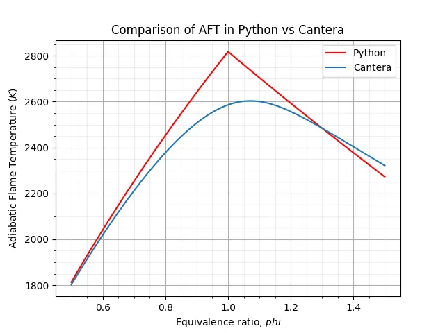
- The equivalence ratio is varied from 0.5 to 1.5 as these are the commonly used values in practice.
- From the graph, we observe the maximum value of AFT = 2817.83 K at phi = 1, because python does not consider all the species in the mixture.

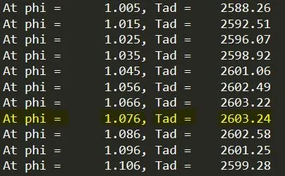
- Cantera gives the maximum AFT = 2603.24 K at phi = 1.076, which is less than in python, as it considers all the species involved in the reaction. Hence, we can say that it is more practical.
***************************************************************************************************************************
Case 2: VARIATION OF ADIABATIC FLAME TEMPERATURE WITH HEAT LOSS AT CONSTANT PRESSURE
The constant pressure adiabatic flame temperature is the temperature that results from a complete combustion process that occurs without any heat transfer or changes in kinetic or potential energy. Its temperature is lower than the constant volume process because some of the energy is utilized to change the volume of the system. In this process, all the heat added goes into changing the volume (expansion) of the gas i.e. work is done by the gas. (W = PΔV)
The maximum possible heat loss is calculated using the Lower Heating Value. The heat loss factor is varied from no heat loss to maximum heat loss.
From First Law,
dU = dQ - PΔV (1)
Also enthalpy (H = U + PV) at constant presure -
ΔH = ΔU + PΔV (2)
Since the process is adiabatic, dQ = 0, therefore,
dU = -PΔV,
Putting this in equation (2),
ΔH = 0
Hence, the required equation is -
HProducts – HReactants + (H_loss*Q) = 0
Code:
"""
AFT of Methane with Heat Loss

# Inputs

fuel = CH4
Condition = Constant Pressure
HHV = 55.5 MJ/kg
LHV = 50 MJ/kg
MW = 16.04 g/mol
N_fuel = 1mol
m_fuel = 16.04 gm
phi = 1

"""

import matplotlib.pyplot as plt
import math
import numpy as np
import cantera as ct


x = 1
y = 4
R = 8.314
Q = 802000 # J/mol, Q = LHV * m_fuel = 50*e*6*16.04*e-03
H_loss = np.linspace(0,1,21)
H_products = []
H_reactants = []

# Function to calculate the enthalpy using NASA polynomial function

def h(T, co_effs):

	R = 8.314 #J/mol-K
	a1 = co_effs[0]
	a2 = co_effs[1]
	a3 = co_effs[2]
	a4 = co_effs[3]
	a5 = co_effs[4]
	a6 = co_effs[5]

	return(a1 + a2*T/2 + a3*pow(T,2)/3 + a4*pow(T,3)/4 + a5*pow(T,4)/5 +a6/T)*R*T

# Low temp coefficients (reactants) at STP condns

CH4_coeffs_l = [5.14987613E+00, -1.36709788E-02, 4.91800599E-05, -4.84743026E-08, 1.66693956E-11, -1.02466476E+04, -4.64130376E+00]

O2_coeffs_l = [3.78245636E+00, -2.99673416E-03, 9.84730201E-06, -9.68129509E-09, 3.24372837E-12, -1.06394356E+03, 3.65767573E+00]

N2_coeffs_l = [0.03298677E+02, 0.14082404E-02, -0.03963222E-04, 0.05641515E-07, -0.02444854E-10, -0.10208999E+04, 0.03950372E+02]

# High temp coefficients (products)

N2_coeffs_h = [0.02926640E+02, 0.14879768E-02, -0.05684760E-05, 0.10097038E-09, -0.06753351E-13, -0.09227977E+04, 0.05980528E+02]

CO2_coeffs_h = [3.85746029E+00, 4.41437026E-03, -2.21481404E-06, 5.23490188E-10, -4.72084164E-14, -4.87591660E+04, 2.27163806E+00]

H20_coeffs_h = [3.03399249E+00, 2.17691804E-03, -1.64072518E-07, -9.70419870E-11, 1.68200992E-14, -3.00042971E+04, 4.96677010E+00]

O2_coeffs_h = [3.28253784E+00, 1.48308754E-03, -7.57966669E-07, 2.09470555E-10, -2.16717794E-14, -1.08845772E+03, 5.45323129E+00]

CO_effs_h = [2.71518561E+00, 2.06252743E-03, -9.98825771E-07, 2.30053008E-10, -2.03647716E-14, -1.41518724E+04, 7.81868772E+00]

# Function for root-solving using NR method iteratively

def f(T, H_loss):

	h_CO2_p = h(T,CO2_coeffs_h)
	h_N2_p = h(T,N2_coeffs_h)
	h_H2O_p = h(T,H20_coeffs_h)

	H_products = h_CO2_p + 2*h_H2O_p + 7.52*h_N2_p

	Tstd = 298.15
	h_CH4_r = h(Tstd, CH4_coeffs_l)
	h_O2_r = h(Tstd, O2_coeffs_l)
	h_N2_r = h(Tstd, N2_coeffs_l)

	H_reactants = h_CH4_r + 2*h_O2_r + 7.52*h_N2_r

	return H_products-H_reactants + (H_loss*Q)

# Defining the derivative of the function

def fprime(T,H_loss):
	return(f(T+1e-6,H_loss) - f(T,H_loss))/1e-6

T_guess = 1500
tol = 1e-3
alpha = 0.9
temp = []

for i in H_loss:

	T_guess = 1500
	R = 8.314

	while(abs(f(T_guess,i)) > tol):
		T_guess = T_guess - alpha*((f(T_guess,i)/fprime(T_guess,i)))

	temp.append(T_guess)

print(max(temp))
print(min(temp))
print(temp)


plt.figure()
plt.plot(H_loss,temp,color='red')
plt.xlabel('Heat-Loss co-efficients')
plt.ylabel('Adiabatic Flame Temperature')
plt.title('Variation of AFT with Heat-Loss co-efficients')
plt.grid(which = 'major')
plt.minorticks_on()
plt.grid(which = 'minor', alpha = 0.2)
plt.show()
RESULTS & DISCUSSION:
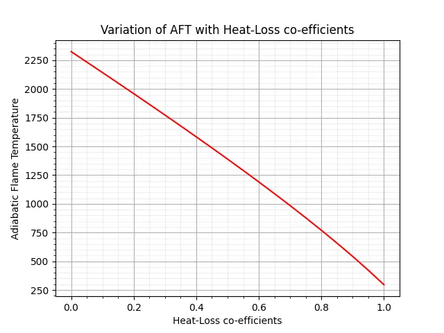
- From the above graph, it is observed that the AFT varies linearly with the heat loss coefficient. The heat released from the reaction is used to increase the flame temperature of the products.
- AFT is maximum (2325.59K) when the heat loss is zero, and minimum (296.06K) when the heat loss is maximum.

- The AFT is 1679K for the heat loss coefficient of 0.35.
***************************************************************************************************************************
Case 3: Variation of Adiabatic Flame Temperature with Alkane, Alkene and Alkyne (2 Carbon atoms)
The number of carbon atoms considered here is 2, which gives the hydrocarbons Ethane (C2H6), Ethene (C2H4) and Ethyne (C2H2).
General Hydrocarbon: CxHy + [x+(y/4)](O2 + 3.76N2) = xCO2 + (y/2)H2O + 3.76[x+(y/4)]N2
Ethane: C2H6 + 3.5(O2 + 3.76N2) = 2CO2 + 3H2O + 13.16N2
Ethene: C2H4 + 3(O2 + 3.76N2) = 2CO2 + 2H20 + 11.28N2
Ethyne: C2H2 + 2.5(O2 + 3.76N2) = 2CO2 + H20 + 9.4 N2
Code:
"""
AFT variation with alkane, alkene, alkyne

General Hydrocarbon: CxHy + [x+(y/4)](O2 + 3.76N2) = xCO2 + (y/2)H2O + 3.76[x+(y/4)]N2

Ethane: C2H6 + 3.5(O2 + 3.76N2) -> 2CO2 + 3H2O  + 13.16N2
Ethene: C2H4 + 3(O2 + 3.76N2) -> 2CO2 + 2H20 + 11.28N2
Ethyne: C2H2 + 2.5(O2 + 3.76N2) -> 2CO2 + H20 + 9.4 N2

"""
import matplotlib.pyplot as plt
import math
import numpy as np
import cantera as ct

# Function to calculate the enthalpy using NASA polynomial function

def h(T, co_effs):

	R = 8.314 #J/mol-K
	a1 = co_effs[0]
	a2 = co_effs[1]
	a3 = co_effs[2]
	a4 = co_effs[3]
	a5 = co_effs[4]
	a6 = co_effs[5]

	return(a1 + a2*T/2 + a3*pow(T,2)/3 + a4*pow(T,3)/4 + a5*pow(T,4)/5 +a6/T)*R*T

# Low temp coefficients (reactants) at STP condns

C2H6_coeffs_l = [4.29142492E+00, -5.50154270E-03, 5.99438288E-05, -7.08466285E-08, 2.68685771E-11, -1.15222055E+04, 2.66682316E+00]

C2H4_coeffs_l = [3.95920148E+00, -7.57052247E-03, 5.70990292E-05, -6.91588753E-08, 2.69884373E-11, 5.08977593E+03, 4.09733096E+00]

C2H2_coeffs_l = [8.08681094E-01, 2.33615629E-02, -3.55171815E-05, 2.80152437E-08, -8.50072974E-12, 2.64289807E+04, 1.39397051E+01]

O2_coeffs_l = [3.78245636E+00, -2.99673416E-03, 9.84730201E-06, -9.68129509E-09, 3.24372837E-12, -1.06394356E+03, 3.65767573E+00]

N2_coeffs_l = [0.03298677E+02, 0.14082404E-02, -0.03963222E-04, 0.05641515E-07, -0.02444854E-10, -0.10208999E+04, 0.03950372E+02]

# High temp coefficients (products)
N2_coeffs_h = [0.02926640E+02, 0.14879768E-02, -0.05684760E-05, 0.10097038E-09, -0.06753351E-13, -0.09227977E+04, 0.05980528E+02]

CO2_coeffs_h = [3.85746029E+00, 4.41437026E-03, -2.21481404E-06, 5.23490188E-10, -4.72084164E-14, -4.87591660E+04, 2.27163806E+00]

H20_coeffs_h = [3.03399249E+00, 2.17691804E-03, -1.64072518E-07, -9.70419870E-11, 1.68200992E-14, -3.00042971E+04, 4.96677010E+00]


Tstp = 298.15 #K

# Function for root-solving using NR method iteratively

def f(T, H_type):
	h_C2H6_r = h(Tstp, C2H6_coeffs_l)
	h_C2H4_r = h(Tstp, C2H4_coeffs_l)
	h_C2H2_r = h(Tstp, C2H2_coeffs_l)
	h_O2_r = h(Tstp, O2_coeffs_l)
	h_N2_r = h(Tstp, N2_coeffs_l)
	h_CO2_p = h(T, CO2_coeffs_h)
	h_N2_p = h(T,N2_coeffs_h)
	h_H2O_p = h(T,H20_coeffs_h)

	if H_type==1:
		x = 2
		y = 6
		H = h_C2H6_r
	elif H_type==2:
		x=2
		y=4
		H = h_C2H4_r
	elif H_type==3:
		x=2
		y=2
		H = h_C2H2_r

	H_reactants = H + (x+y/4)*(h_O2_r + 3.76*h_N2_r)
	H_products = x*h_CO2_p + (y/2)*h_H2O_p + 3.76*(x+y/4)*h_N2_p

	return H_products - H_reactants

# Defining the derivative of the function

def fprime(T, H_type):
	return(f(T+1e-6,H_type) - f(T,H_type))/1e-6

alpha = 1
T_guess = 1500
tol = 1e-3
H_type = [1, 2, 3]
temp = []

for i in range(0,len(H_type)):

	T_guess = 1500
	R = 8.314

	while(abs(f(T_guess,H_type[i])) > tol):
		T_guess = T_guess - alpha*((f(T_guess,H_type[i])/fprime(T_guess,H_type[i])))

	temp.append(T_guess)

print(max(temp))
print(temp)


plt.bar(['Ethane $C_2H_6$', 'Ethene $C_2H_4$', 'Ethyne $C_2H_2$'], temp)
plt.ylabel('Adiabatic Flame Temperature ($K$)')
plt.title('Variation of AFT with Hyrdrocarbons (Python)')
plt.show()

################################################################################

#Solution using Cantera

gas = ct.Solution('gri30.xml')
gas.TPX = 298.15, 101325, {'C2H6':1, 'O2':3.5, 'N2':13.16}
gas.equilibrate('HP','auto')
T_C2H6 = gas.T

gas.TPX = 298.15, 101325, {'C2H4':1, 'O2':3, 'N2':11.28}
gas.equilibrate('HP','auto')
T_C2H4 = gas.T

gas.TPX = 298.15, 101325, {'C2H2':1, 'O2':2.5, 'N2':9.4}
gas.equilibrate('HP','auto')
T_C2H2 = gas.T

temp = (T_C2H6, T_C2H4, T_C2H2)

temp = np.array(temp)
print(temp)

plt.bar(['Ethane $C_2H_6$','Ethene $C_2H_4$','Ethyne $C_2H_2$'], temp, color='green')
plt.ylabel('Adiabatic Flame Temperature ($K$)')
plt.title('Variation of AFT with Hydrocarbons (Cantera)')
plt.show()
RESULTS & DISCUSSION:
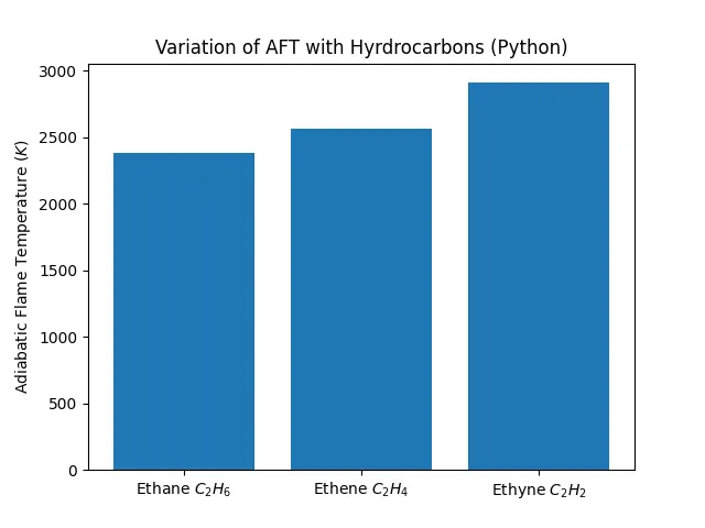
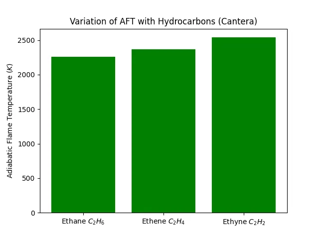
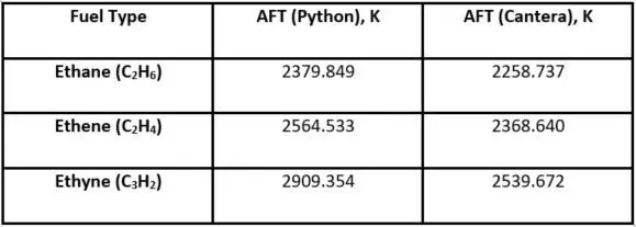
- Alkyne i.e. Ethyne shows the highest temperature (2909.35K in Python and 2539.67K in Cantera) followed by alkene (Ethene) and alkane (Ethane). This is due to the presence of triple bonds and double bonds in ethyne and ethene respectively.
- The temperature trend is the same for python and cantera, but the temperature values are lower for cantera as it solves for all the species.
*********************************************************************************************************************
Case 4: VARIATION OF ADIABATIC FLAME TEMPERATURE WITH ALKANE FOR CARBON ATOM CHAINS (1-3)
The final study is done for alkane with carbon atoms varying from 1 to 3. The combustion equations for the hydrocarbons are as follows -
Methane: CH4 + 2(O2 + 3.76N2) = CO2 + 2H2O + 7.52N2
Ethane: C2H6 + 3.5(O2 + 3.76N2) = 2CO2 + 3H2O + 13.16N2
Propane: C3H8 + 5(O2 + 3.76N2) = 3CO2 + 4H20 + 18.8N2
Code:
"""
AFT variation w.r.t a number of carbon atom chains

General Hydrocarbon:

CxHy + [x+(y/4)](O2 + 3.76N2) = xCO2 + (y/2)H2O + 3.76[x+(y/4)]N2

Methane: CH4 + 2(O2 + 3.76N2) = CO2 + 2H2O + 7.52N2
Ethane: C2H6 + 3.5(O2 + 3.76N2) = 2CO2 + 3H2O  + 13.16N2
Propane: C3H8 + 5(O2 + 3.76N2) = 3CO2 + 4H20 + 18.8N2

"""
import matplotlib.pyplot as plt
import math
import numpy as np
import cantera as ct


# Function to calculate the enthalpy using NASA polynomial function

def h(T, co_effs):

	R = 8.314 #J/mol-K
	a1 = co_effs[0]
	a2 = co_effs[1]
	a3 = co_effs[2]
	a4 = co_effs[3]
	a5 = co_effs[4]
	a6 = co_effs[5]

	return(a1 + a2*T/2 + a3*pow(T,2)/3 + a4*pow(T,3)/4 + a5*pow(T,4)/5 +a6/T)*R*T

# Low temp coefficients (reactants) at STP condns

CH4_coeffs_l = [5.14987613E+00, -1.36709788E-02, 4.91800599E-05, -4.84743026E-08, 1.66693956E-11, -1.02466476E+04, -4.64130376E+00]

C2H6_coeffs_l = [4.29142492E+00, -5.50154270E-03, 5.99438288E-05, -7.08466285E-08, 2.68685771E-11, -1.15222055E+04, 2.66682316E+00]

C3H8_coeffs_l = [0.93355381E+00, 0.26424579E-01, 0.61059727E-05, -0.21977499E-07, 0.95149253E-11, -0.13958520E+05, 0.19201691E+02]

O2_coeffs_l = [3.78245636E+00, -2.99673416E-03, 9.84730201E-06, -9.68129509E-09, 3.24372837E-12, -1.06394356E+03, 3.65767573E+00]

N2_coeffs_l = [0.03298677E+02, 0.14082404E-02, -0.03963222E-04, 0.05641515E-07, -0.02444854E-10, -0.10208999E+04, 0.03950372E+02]

# High temp coeff (products)

N2_coeffs_h = [0.02926640E+02, 0.14879768E-02, -0.05684760E-05, 0.10097038E-09, -0.06753351E-13, -0.09227977E+04, 0.05980528E+02]

CO2_coeffs_h = [3.85746029E+00, 4.41437026E-03, -2.21481404E-06, 5.23490188E-10, -4.72084164E-14, -4.87591660E+04, 2.27163806E+00]

H20_coeffs_h = [3.03399249E+00, 2.17691804E-03, -1.64072518E-07, -9.70419870E-11, 1.68200992E-14, -3.00042971E+04, 4.96677010E+00]


Tstp = 298.15 #K

# Function for root-solving using NR method iteratively

def f(T, H_type):

	h_CH4_r = h(Tstp, CH4_coeffs_l)
	h_C2H6_r = h(Tstp, C2H6_coeffs_l)
	h_C3H8_r = h(Tstp, C3H8_coeffs_l)
	h_O2_r = h(Tstp, O2_coeffs_l)
	h_N2_r = h(Tstp, N2_coeffs_l)
	h_CO2_p = h(Tstp, CO2_coeffs_h)
	h_N2_p = h(T,N2_coeffs_h)
	h_H2O_p = h(T,H20_coeffs_h)

	if H_type==1:
		x = 1
		y = 4
		H = h_CH4_r
	elif H_type==2:
		x=2
		y=6
		H = h_C2H6_r
	elif H_type==3:
		x=3
		y=8
		H = h_C3H8_r

	H_reactants = H + (x+y/4)*(h_O2_r + 3.76*h_N2_r)
	H_products = x*h_CO2_p + (y/2)*h_H2O_p + 3.76*(x+y/4)*h_N2_p

	return H_products - H_reactants

# Defining the derivative of the function

def fprime(T, H_type):
	return(f(T+1e-6,H_type) - f(T,H_type))/1e-6

alpha = 1
T_guess = 1500
tol = 1e-3
H_type = [1, 2, 3]
temp = []

for i in range(0,len(H_type)):

	T_guess = 1500
	R = 8.314

	while(abs(f(T_guess,H_type[i])) > tol):
		T_guess = T_guess - alpha*((f(T_guess,H_type[i])/fprime(T_guess,H_type[i])))

	temp.append(T_guess)

print(max(temp))
print(temp)

# Plotting

plt.bar(['Methane $CH_4$', 'Ethane $C_2H_6$', 'Propane $C_3H_8$'], temp)
plt.ylabel('Adiabatic Flame Temperature ($K$)')
plt.title('Variation of AFT with number of Carbon (Python)')
plt.show()

###########################################################################

# Solution using Cantera

gas = ct.Solution('gri30.xml')
gas.TPX = 298.15, 101325, {'CH4':1, 'O2':2, 'N2':7.52}
gas.equilibrate('HP','auto')
T_CH4 = gas.T

gas.TPX = 298.15, 101325, {'C2H6':1, 'O2':3.5, 'N2':13.16}
gas.equilibrate('HP','auto')
T_C2H6 = gas.T

gas.TPX = 298.15, 101325, {'C3H8':1, 'O2':5, 'N2':18.8}
gas.equilibrate('HP','auto')
T_C3H8 = gas.T

temp = (T_CH4, T_C2H6, T_C3H8)

temp = np.array(temp)
print(temp)

#Plotting

plt.bar(['Methane $CH_4$','Ethane $C_2H_6$','Propane $C_3H_8$'], temp, color='green')
plt.ylabel('Adiabatic Flame Temperature ($K$)')
plt.title('Variation of AFT with number of Carbon (Cantera)')
plt.show()
RESULTS & DISCUSSION:
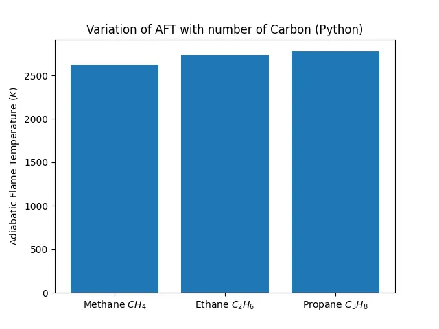
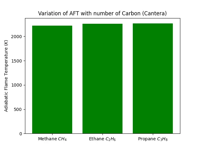
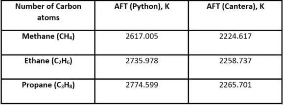
- Owing to more number of carbon atoms the fuel Propane gives the maximum temperature (2774.59K in Python and 2265.70K in Cantera) followed by Ethane and Methane.
- The temperatures are lower in Cantera as it solves for all the species. Moreover, the temperature differences are also smaller in Cantera as compared to Python.