Week 3 - Adiabatic Flame Temperature calculation
Aim:
The aim of this project is to simulate the combustion of methane for the calculation of AFT.
Objectives:
- Effect of equivalence ratio on AFT.
- Constant pressure process with heat loss parameters.
- AFT variation with respect to an alkane, alkyne, and alkene.
- Testing the different fuels with 2 carbon atom bonds.
Adiabatic flame temperature(AFT):-
In the study of combustion, there are two types of adiabatic flame temperature depending on how the process is completed: the constant volume and the constant pressure; both of which describe temperature that combustion products theoretically can reach if there is no energy is lost to the outside environment.
The constant volume adiabatic flame temperature is the temperature that results from a complete combustion process that occurs without any work, heat transfer or changes in kinetic or potential energy. Its temperature is higher than the constant pressure process because no energy is utilized to change the volume of the system (i.e., generate work).
AFT is going to calculated by using the Newton-Raphson iterative method to find the root of the function using an initial guess value and it iterates until it reaches the given tolerance value.
Tnew = `T_(guess) - alpha* [f(T_(guess))/(f'(T_(guess)))]`
1) AFT variation with Equivalence ratio varying with Cantera.
A stoichiometric mixture of combustion of methane looks like as following:
`CH_4 + 2(O_2+3.76N_2) to CO_2 + 2H_2O + 7.52N_2`
The general reaction for any fuel is given below:
`C_xH_y+(x+y/4)(O_2+3.76N_2)toxCO_2+y/2H_2O+(x+y/4)N_2`
But the combustion is not always stoichiometric. It can be either lean combustion or rich combustion.
Lean mixture`phi` < 1:
`CH + 2/phi(O_2+3.76N_2) to CO_2+H_2O+(2/phi-2)O_2+7.52/phiN_2`
Rich mixture`phi` > 1:-
`CH_4+2/phi(O_2+3.76N_2)to(4/phi-3)CO_2+2H_2O+(4/phi-4)CO+7.52/phiN_2`
Code:
import matplotlib.pyplot as plt
import numpy as np
import cantera as ct

# Function defining temperature and coefficients
def h(T, coeff):

	R = 8.314	# J/mol-K
	a1 = coeff[0]
	a2 = coeff[1]
	a3 = coeff[2]
	a4 = coeff[3]
	a5 = coeff[4]
	a6 = coeff[5]

	return (a1 + a2*T/2 + a3*pow(T,2)/3 + a4*pow(T,3)/4 + a5*pow(T,4)/5 + a6/T)*R*T


# Defining the NASA coefficients from datsheet of reactants (low temperature)

ch4_coeff_l = [5.14987613E+00, -1.36709788E-02, 4.91800599E-05, -4.84743026E-08, 1.66693956E-11, -1.02466476E+04, -4.64130376E+00]

o2_coeff_l = [3.78245636E+00, -2.99673416E-03, 9.84730201E-06, -9.68129509E-09, 3.24372837E-12, -1.06394356E+03, 3.65767573E+00]

n2_coeff_l = [0.03298677E+02, 0.14082404E-02, -0.03963222E-04, 0.05641515E-07, -0.02444854E-10, -0.10208999E+04, 0.03950372E+02]


# Defining the NASA coefficients from datsheet of reactants (high temperature)

co2_coeff_h = [3.85746029E+00, 4.41437026E-03, -2.21481404E-06, 5.23490188E-10, -4.72084164E-14, -4.87591660E+04, 2.27163806E+00]

h2o_coeff_h = [3.03399249E+00, 2.17691804E-03, -1.64072518E-07, -9.70419870E-11, 1.68200992E-14, -3.00042971E+04, 4.96677010E+00]

n2_coeff_h = [0.02926640E+02, 0.14879768E-02, -0.05684760E-05, 0.10097038E-09, -0.06753351E-13, -0.09227977E+04, 0.05980528E+02]

co_coeff_h = [2.71518561E+00, 2.06252743E-03, -9.98825771E-07, 2.30053008E-10, -2.03647716E-14, -1.41518724E+04, 7.81868772E+00]

o2_coeff_h =  [3.28253784E+00, 1.48308754E-03, -7.57966669E-07, 2.09470555E-10, -2.16717794E-14, -1.08845772E+03, 5.45323129E+00]


# Defining the function for root-solving by Newton-Raphson method

def f(T, phi):

	Tstp =298.15 # Temperature of the reactants in Kelvin
	R= 8.314 #Jol/ mol-k
	h_ch4_r = h(Tstp, ch4_coeff_l)
	h_o2_r = h(Tstp, o2_coeff_l)
	h_n2_r = h(Tstp, n2_coeff_l)

	H_reactants = h_ch4_r + (2/phi)*h_o2_r + (7.52/phi)*h_n2_r
	N_reactants = (1 + (2/phi) + (7.52/phi))*R*Tstp

	h_co2_p = h(T, co2_coeff_h)
	h_h2o_p = h(T, h2o_coeff_h)
	h_n2_p = h(T, n2_coeff_h)
	h_co_p = h(T, co_coeff_h)
	h_o2_p = h(T, o2_coeff_h)

	if phi >= 1:
		H_products = (4/phi-3)*h_co2_p + 2*h_h2o_p + (7.52/phi)*h_n2_p + (4-4/phi)*h_co_p
		N_products = ((4/phi - 3) + 2 + (7.52/phi) + (4-4/phi))*R*T
	elif phi < 1:
		H_products = h_co2_p + 2*h_h2o_p + (7.52/phi)*h_n2_p + (2/phi-2)*h_o2_p
		N_products = (1 + 2 + (7.52/phi) + (2/phi-2))*R*T

	return (H_products - H_reactants) - (N_products - N_reactants)
#Since reaction is in a constant volume chamber no. of moles are also added


def fprime(T, phi):
	return (f(T+1e-6, phi) - f(T, phi))/(1e-6)

# Defining Newton-Raphson solver

alpha = 0.2
tol = 1e-3
phi = [0.1, 0.2, 0.3, 0.4, 0.5, 0.6, 0.7, 0.8, 0.9, 1, 1.1, 1.2, 1.3, 1.4, 1.5, 1.6, 1.7, 1.8, 1.9, 2]
T_aft_py = []

for i in range(0,len(phi)):
	T_guess = 1500	# K
	while abs(f(T_guess, phi[i])) >= tol:
		T_guess = T_guess - alpha*((f(T_guess, phi[i]))/(fprime(T_guess, phi[i])))
	T_aft_py.append(T_guess)
print(T_aft_py)
print()

#Solution obtained by Cantera

gas = ct.Solution("gri30.xml")
T_aft_ct = []

for i in range(0,len(phi)):
	# Computing the mole fractions of each reactant
	n_tot = 1 + (2/phi[i]) + (7.52/phi[i])
	n_ch4 = 1/n_tot
	n_o2 = (2/phi[i])/n_tot
	n_n2 = (7.52/phi[i])/n_tot
	# Defining the gas mixture
	gas.TPX = 298.15, 101325, {'CH4':n_ch4, 'O2':n_o2, 'N2':n_n2}
	# Calculating the equilibrium conditions
	gas.equilibrate('UV','auto')
	T_aft_ct.append(gas.T)
print(T_aft_ct)


# Plotting
plt.plot(phi,T_aft_py,'-o',color='red',label='Python', linewidth='2')
plt.plot(phi, T_aft_ct, '-o',color='blue',label='Cantera')
plt.xlabel('Equivalence Ratio ($phi$)', fontsize=10)
plt.ylabel('Adiabatic Flame Temperature [K]', fontsize=10)
plt.yticks(np.arange(0, 3000, step=200))
plt.xticks(np.arange(0, 2, step=0.15))
plt.grid('on')
plt.title('AFT vs. Equivalence Ratio for Methane-Air Combustion', fontsize=12, fontweight='bold')
plt.legend(fontsize=14)
plt.show()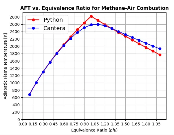
2) AFT variation with heat loss:
In this objective, heat loss is involved. So, this is not an adiabatic process. Hence enthalpy calculation includes a lower heating value.
`CH_4 + 2(O_2+3.76N_2) to CO_2 + 2H_2O + 7.52N_2`
H.V = `h_(f,CH_4)^298 + 2h_(f,O_2)^298 - h_(f,CO_2)^298-2h_(f,H_2O)^298` , Nitrogen is cancelled.
Code:
import numpy as np
import cantera as ct
import matplotlib.pyplot as plt


# Stoichiometric reaction :- CH4 +2(O2+3.76N2) -> CO2 +2H2O +7.52N2
# Function defining temperature and coefficients

def h(T,coeffs):


	R=8.314 #J/mol-K
	a1=coeffs[0]
	a2=coeffs[1]
	a3=coeffs[2]
	a4=coeffs[3]
	a5=coeffs[4]
	a6=coeffs[5]

	return (a1+a2*T/2+a3*pow(T,2)/3+a4*pow(T,3)/4+a5*pow(T,4)/5+a6/T)*R*T

# Defining the NASA coefficients from datsheet of reactants (low temperature)

ch4_coef_l=[5.14987613E+00,-1.36709788E-02, 4.91800599E-05, -4.84743026E-08, 1.66693956E-11,-1.02466476E+04,-4.64130376E+00]

o2_coef_l=[3.78245636E+00,-2.99673416E-03, 9.84730201E-06, -9.68129509E-09, 3.24372837E-12,-1.06394356E+03, 3.65767573E+00]

n2_coef_l=[0.03298677E+02, 0.14082404E-02,-0.03963222E-04,0.05641515E-07,-0.02444854E-10,-0.10208999E+04, 0.03950372E+02]


# Defining the NASA coefficients from datsheet of reactants (high temperature)

n2_coef_h=[0.02926640E+02, 0.14879768E-02,-0.05684760E-05, 0.10097038E-09,-0.06753351E-13,-0.09227977E+04, 0.05980528E+02]

h2o_coef_h=[3.03399249E+00, 2.17691804E-03,-1.64072518E-07,-9.70419870E-11, 1.68200992E-14,-3.00042971E+04, 4.96677010E+00 ]

co2_coef_h=[3.85746029E+00, 4.41437026E-03,-2.21481404E-06, 5.23490188E-10,-4.72084164E-14,-4.87591660E+04, 2.27163806E+00]


# Computing the maximum possible heat loss
Tstd=298.15
# Nitrogen gets cancelled as has same moles in reactant and products side
LHV = h(Tstd,ch4_coef_l) + 2*h(Tstd,o2_coef_l) - h(Tstd,co2_coef_h)- 2*h(Tstd,h2o_coef_h)

# evaluation of enthalpy

def f(T,H_loss):
	Tstd=298.15

	#enthalpy of products
	h_co2_p= h(T,co2_coef_h)
	h_h2o_p= h(T,h2o_coef_h)
	h_n2_p= h(T,n2_coef_h)
	H_p=h_co2_p+2*h_h2o_p+7.52*h_n2_p
	#print(H_p)

	# enthalpy of reactants

	h_ch4_r=h(Tstd,ch4_coef_l)
	h_o2_r= h(Tstd,o2_coef_l)
	h_n2_r= h(Tstd,n2_coef_l)
	H_r=h_ch4_r+2*h_o2_r+7.52*h_n2_r
	#print(H_r)

	print(LHV)
	return H_p-H_r+(H_loss*LHV)


def fprime(T):
	return (f(T+1e-6,H_loss) - f(T,H_loss))/1e-6

H_loss=0
T_aft=[]
H_l=[]

while(H_loss<1):
	T_g=1500
	tol=1e-4
	alpha=1
	ct=0

# Newton raphson technique
	while(abs(f(T_g,H_loss))>tol):
		T_g=T_g- alpha*((f(T_g,H_loss)/fprime(T_g)))
		ct=ct+1
	plt.plot(H_loss,T_g,'*',color='black')
	H_l.append(H_loss)
	H_loss=H_loss+0.1
	T_aft.append(T_g)

# plotting

plt.plot(H_l,T_aft,color='red',linewidth=1.5)
plt.xlabel('Heat Loss Fraction')
plt.ylabel('Flame Temperture(K)')
plt.title('Flame Temperture vs Heat Loss Fraction')
plt.grid(True)
plt.show()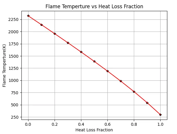
3) Adiabatic flame temperature variation with respect to Alkane, Alkene, Alkyne :
Here in the combustion process ethane, ethyne, and ethene are involved. The reactions are given below:
Ethane:- `C_2H_6 + 3.5(O_2+3.76N_2) to 2CO_2 + 3H_2O+13.16N_2`
Ethene:- `C_2H_4 + 3(O_2+3.76N_2) to 2CO_2 + 2H_2O+11.28N_2`
Ethyne:- `C_2H_2 + 2.5(O_2+3.76N_2) to 2CO_2 + H_2O+9.4N_2`
The combustion is again in constant pressure chamber with heat loss factor = 0.35.
Hence the equilibrium reaction is H_products - H_reactants + 0.35 * L.H.V = 0.
Code:
"AFT Variation with respect to alk-ane,ene,yne with same no. of two Carbon atom chain"
import numpy as np
import cantera as ct
import matplotlib.pyplot as plt

def h(T,coeffs):
	#evaluation of enthalpy
	R=8.314 #J/mol-K
	a1 = coeffs[0]
	a2 = coeffs[1]
	a3 = coeffs[2]
	a4 = coeffs[3]
	a5 = coeffs[4]
	a6 = coeffs[5]

	return (a1+a2*T/2+a3*pow(T,2)/3+a4*pow(T,3)/4+a5*pow(T,4)/5+a6/T)*R*T

c2h6_coef_l = [4.29142492E+00,-5.50154270E-03, 5.99438288E-05,-7.08466285E-08, 2.68685771E-11,-1.15222055E+04, 2.66682316E+00]
c2h4_coef_l = [3.95920148E+00,-7.57052247E-03, 5.70990292E-05,-6.91588753E-08, 2.69884373E-11, 5.08977593E+03, 4.09733096E+00 ]
c2h2_coef_l = [8.08681094E-01, 2.33615629E-02,-3.55171815E-05, 2.80152437E-08,-8.50072974E-12, 2.64289807E+04, 1.39397051E+01]
o2_coef_l = [3.78245636E+00,-2.99673416E-03, 9.84730201E-06, -9.68129509E-09, 3.24372837E-12,-1.06394356E+03, 3.65767573E+00]
n2_coef_l = [0.03298677E+02, 0.14082404E-02,-0.03963222E-04,0.05641515E-07,-0.02444854E-10,-0.10208999E+04, 0.03950372E+02]
n2_coef_h = [0.02926640E+02, 0.14879768E-02,-0.05684760E-05, 0.10097038E-09,-0.06753351E-13,-0.09227977E+04, 0.05980528E+02]
h2o_coef_h = [3.03399249E+00, 2.17691804E-03,-1.64072518E-07,-9.70419870E-11, 1.68200992E-14,-3.00042971E+04, 4.96677010E+00]
co2_coef_h = [3.85746029E+00, 4.41437026E-03,-2.21481404E-06, 5.23490188E-10,-4.72084164E-14,-4.87591660E+04, 2.27163806E+00]

# The standard reaction :- CxHy+(x + y/4)(O2+3.76N2) -> xCO2+y/2H2O+(x + y/4)3.76N2
# We know that x=2 as carbon atom chain is fixed and y=6(Ethane) ; y=4(Ethene) ; y=2(Ethyne)

def f(T,y):
	Tstd = 298.15
	H_loss = 0.35
	x = 2
	if y == 6:                           #(Ethane)
		h_fuel_r=h(Tstd,c2h6_coef_l)
	elif y==4:                         #(Ethene)
		h_fuel_r=h(Tstd,c2h4_coef_l)
	else :                             #(Ethyne)
		h_fuel_r=h(Tstd,c2h2_coef_l)

	#products at STP
	h_co2_p = h(Tstd,co2_coef_h)
	h_h2o_p = h(Tstd,h2o_coef_h)
	h_n2_p = h(Tstd,n2_coef_h)
	H_p_s = x*h_co2_p+(y/2)*h_h2o_p+3.76*(x + y/4)*h_n2_p

	#enthalpy of products
	h_co2_p = h(T,co2_coef_h)
	h_h2o_p = h(T,h2o_coef_h)
	h_n2_p = h(T,n2_coef_h)
	H_p = x*h_co2_p+(y/2)*h_h2o_p+3.76*(x + y/4)*h_n2_p
	#print(H_p)

	#enthalpy of reactants

	#h_fuel_r=h(Tstd,f_coef_l)
	h_o2_r = h(Tstd,o2_coef_l)
	h_n2_r = h(Tstd,n2_coef_l)
	H_r = h_fuel_r+(x + y/4)*h_o2_r+3.6*(x + y/4)*h_n2_r
	#print(H_r)
	LHV = H_r-H_p_s
	#print(LHV)
	return H_p-H_r+(H_loss*LHV)

dt = 1e-4
def fprime(T):
	return (f(T+1e-6,y) - f(T,y))/1e-6

T_aft = []

for y in range (6,0,-2):
	T_g = 1500
#Newton raphson technique
	tol = 1e-4
	alpha = 0.2
	ct = 0
	while (abs(f(T_g,y))>tol):
		T_g = T_g- alpha*((f(T_g,y)/fprime(T_g)))
		ct = ct+1

	T_aft.append(T_g)

fuel = ['Ethane', 'Ethene', 'Ethyne']
fuel_pos = [i for i, _ in enumerate(fuel)]

fig, ax = plt.subplots()
bars = ax.bar(fuel_pos, T_aft, width=0.4, color='blue')
for bar in bars:
        height = bar.get_height()
        ax.text(bar.get_x() + bar.get_width()/2., 1.05*height,
                '%f' % float(height),
        ha='center', va='bottom')
plt.xlabel('Hydrocarbon Type')
plt.ylabel('Adiabatic Flame Temperature(K)')
plt.title("AFT for different Hydrocarbons")
plt.xticks(fuel_pos, fuel)
#plt.grid('on')
plt.ylim((0,2350))
plt.show()
Result:
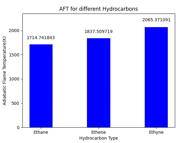
4) Adiabatic flame temperature variation with respect to a number of Carbon atom chains :
Here the combustion process involves methane, ethane, and propane, and their reactions are shown below:
Methane:- `CH_4 + 2(O_2+3.76N_2) to CO_2 + 2H_2O + 7.52N_2`
Ethane:- `C_2H_6 + 3.5(O_2+3.76N_2) to 2CO_2 + 3H_2O + 13.16N_2`
Propane:- `C_3H_8 + 5(O_2+3.76N_2) to 3CO_2 + 4H_2O + 18.8N_2`
Equilibrium reaction:- H_products - H_reactants = 0
Code:
"AFT Variation with respect to number of Carbon atom chains"

import matplotlib.pyplot as plt
import numpy as np
import cantera as ct


def h(T,Coeff):
	R= 8.314
	a1=Coeff[0]
	a2=Coeff[1]
	a3=Coeff[2]
	a4=Coeff[3]
	a5=Coeff[4]
	a6=Coeff[5]
	a7=Coeff[6]

	return (a1 + a2*T/2 + a3 * pow(T,2)/ 3 + a4 * pow(T,3)/ 4 + a5 * pow(T,4)/ 5 + a6 / T) *R*T

ch4_coeffs_l = [5.14987613E+00,-1.36709788E-02, 4.91800599E-05,-4.84743026E-08, 1.66693956E-11,-1.02466476E+04,-4.64130376E+00]

c2h6_coeffs_l =[4.29142492E+00,-5.50154270E-03, 5.99438288E-05,-7.08466285E-08 ,2.68685771E-11,-1.15222055E+04 ,2.66682316E+00]

c3h8_coeffs_l =[0.93355381E+00, 0.26424579E-01,0.61059727E-05,-0.21977499E-07 ,0.95149253E-11 ,-0.13958520E+05 ,0.19201691E+02]

n2_coeffs_l  = [0.03298677E+02, 0.14082404E-02,-0.03963222E-04, 0.05641515E-07,-0.02444854E-10,-0.10208999E+04, 0.03950372E+02]

n2_coeffs_h  = [0.02926640E+02, 0.14879768E-02,-0.05684760E-05, 0.10097038E-09,-0.06753351E-13,-0.09227977E+04, 0.05980528E+02]

o2_coeffs_l  = [3.78245636E+00,-2.99673416E-03, 9.84730201E-06,-9.68129509E-09, 3.24372837E-12,-1.06394356E+03, 3.65767573E+00]

co2_coeffs_h = [3.85746029E+00, 4.41437026E-03,-2.21481404E-06, 5.23490188E-10,-4.72084164E-14,-4.87591660E+04, 2.27163806E+00]

h2o_coeffs_h = [3.03399249E+00, 2.17691804E-03,-1.64072518E-07,-9.70419870E-11, 1.68200992E-14,-3.00042971E+04, 4.96677010E+00]

# The standard reaction :- CxHy+(x + y/4)(O2+3.76N2) ---> xCO2+y/2H2O+(x + y/4)3.76N2
# Here we vary the value of n=1(Methane),2(Ethane),3(Propane) where x=2n and y=2n+2
# Methane_reaction :CH4 + 2O2 + 2*3.76 N2 = CO2 + 2H2O + 2*3.76 N2

def f_Methane(T):
	Tstp =298.15

	h_ch4_r= h(Tstp,ch4_coeffs_l)
	h_o2_r= h(Tstp,o2_coeffs_l)
	h_n2_r = h(Tstp,n2_coeffs_l)
	h_n2_p = h(T,n2_coeffs_h)
	h_co2_p = h(T,co2_coeffs_h)
	h_h2o_p = h(T,h2o_coeffs_h)

	h_reactants = h_ch4_r+ 2*h_o2_r +(2*3.76*h_n2_r)
	h_products = h_co2_p+ 2*h_h2o_p +(2*3.76*h_n2_p)

	return h_products - h_reactants

def fprime_Methane(T):
	return (f_Methane(T+ 1e-6)- f_Methane(T))/1e-6

#Ethane_reaction: C2H6 + 3.5O2 +3.5 *3.76 N2 = 2CO2 + 3H2O + 3.5 *3.76 N2
def f_Ethane(T):
	Tstp =298.15

	h_c2h6_r= h(Tstp,c2h6_coeffs_l)
	h_o2_r= h(Tstp,o2_coeffs_l)
	h_n2_r = h(Tstp,n2_coeffs_l)
	h_n2_p = h(T,n2_coeffs_h)
	h_co2_p = h(T,co2_coeffs_h)
	h_h2o_p = h(T,h2o_coeffs_h)

	h_reactants = h_c2h6_r+ 3.5*h_o2_r +(3.5*3.76*h_n2_r)
	h_products= 2*h_co2_p+ 3*h_h2o_p +(3.5*3.76*h_n2_p)

	return h_products - h_reactants

def fprime_Ethane(T):
	return (f_Ethane(T+ 1e-6)- f_Ethane(T))/1e-6

#propane: C3H8 + 5O2 + 5*3.76 N2 = 3CO2 + 4H2O + 5 *3.76 N2

def f_Propane(T):
	Tstp =298.15
	h_c3h8_r= h(Tstp,c3h8_coeffs_l)
	h_o2_r= h(Tstp,o2_coeffs_l)
	h_n2_r = h(Tstp,n2_coeffs_l)
	h_n2_p = h(T,n2_coeffs_h)
	h_co2_p = h(T,co2_coeffs_h)
	h_h2o_p = h(T,h2o_coeffs_h)

	h_reactants = h_c3h8_r+ 5*h_o2_r +(5*3.76*h_n2_r)
	h_products= 3*h_co2_p+ 4*h_h2o_p +(5*3.76*h_n2_p)

	return h_products - h_reactants

def fprime_Propane(T):
	return (f_Propane(T+ 1e-6)- f_Propane(T))/1e-6

T_Methane=1500
T_Ethane=1500
T_Propane=1500
tol = 1e-3
alpha = 1


T_aft=[]

while (abs(f_Methane(T_Methane))>tol):
	T_Methane = T_Methane - alpha*(f_Methane(T_Methane)/fprime_Methane(T_Methane))


T_aft.append(T_Methane)

while (abs(f_Ethane(T_Ethane))>tol):
	T_Ethane = T_Ethane - alpha*(f_Ethane(T_Ethane)/fprime_Ethane(T_Ethane))

T_aft.append(T_Ethane)

while (abs(f_Propane(T_Propane))>tol):
	T_Propane = T_Propane - alpha*(f_Propane(T_Propane)/fprime_Propane(T_Propane))

T_aft.append(T_Propane)

fuel = ['Methane', 'Ethane', 'Propane']
fuel_pos = [i for i, _ in enumerate(fuel)]

fig, ax = plt.subplots()
bars = ax.bar(fuel_pos, T_aft, width=0.4, color='blue')
plt.xlabel('Type of Alkane')
plt.ylabel('Adiabatic Flame Temperature(K)')
plt.title("AFT for different Alkanes")
plt.xticks(fuel_pos, fuel)
plt.ylim((0,2750))
plt.show()
Result:
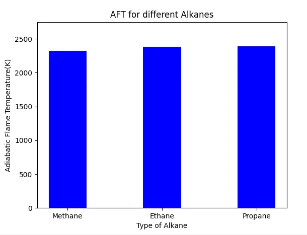
Conclusion:
The effect of the equivalence ratio was observed with AFT. The temperature obtained in python is higher when compared with cantera. From the 2nd objective, it can be said that heat loss fraction increases with a decrease in the flame temperature. From the 3rd objective, we can say that the number of bonds increases hence the AFT is high for a triple bond. From the 4th objective, it is evident that the bar graph of the carbon atoms increases with the AFT increases.