Adiabatic Flame Temperature calculation
AIM
The aim of this project is to simulate the combustion of methane for calculation of Adiabatic Flame Temperature
OBJECTIVES
The main objectives are as follows
- Effect of equivalence ratio on AFT for methane
- Constant pressure process with heat loss parameter
- Testing the different fuels with 2 carbon atom bond
ADIABATIC FLAME TEMPERATURE
In the study of combustion, there are two types of adiabatic flame temperature depending on how the process is completed: the constant volume and constant pressure; both of which describe temperature that combustion products theoretically can reach if no energy is lost to the outside environment.The constant volume adiabatic flame temperature is the temperature that results from a complete combustion process that occurs without any work, heat transfer or changes in kinetic or potential energy. Its temperature is higher than the constant pressure process because no energy is utilized to change the volume of the system.
From the first law of thermodynamics for a closed reacting system we have,

where,  and
and  are the heat and work transferred from the system to the surroundings during the process respectively, and
  and
and  are the internal energy of the reactants and products respectively. In the constant volume adiabatic flame temperature case, the volume of the system is held constant hence there is no work occurring,

and there is no heat transfer because the process is defined to be adiabatic:  . As a result, the internal energy of the products is equal to the internal energy of the reactants:
  . Because this is a closed system, the mass of the products and reactants is constant and the first law can be written on a mass basis,
 .
.
In the constant pressure adiabatic flame temperature case, the pressure of the system is held constant which results in the following equation for the work,

Again there is no heat transfer occurring because the process is defined to be adiabatic: . From the first law, we find that,

Recalling the definition of enthalpy we recover:  . Because this is a closed system, the mass of the products and reactants is constant and the first law can be written on a mass basis,
 .
.
We see that the adiabatic flame temperature of the constant pressure process is lower than that of the constant volume process. This is because some of the energy released during combustion goes into changing the volume of the control system.
COMBUSTION REACTIONS FOR METHANE WITH EQUIVALENCE RATIO
The purpose of combustion is to consume fuel efficiently to produce heat. There are three components of combustion: fuel, oxygen and heat. The most common fuel sources in a combustion process are fossil fuels; natural gas, oil and coal. Fossil fuels are hydrocarbons; organic compounds containing carbon and hydrogen. To maximize the efficiency of combustion, it is vital to consume (or burn) all the fuel, which is known as complete combustion. The reaction for the methane is as follows
`CH_4+2(O_2+3.76N_2)rightarrowCO_2+2H_2O+7.52N_2`
The general reaction for any fuel is given by
`C_xH_y+(x+y/4)(O_2+3.76N_2)rightarrowxCO_2+y/2H_2O+(x+y/4)N2`
Now in order to estimate the effect of equivalence ratio on combustion of methane we consider the balanced reaction for lean and rich mixtures
Lean Mixture `phi<1`
`CH_+2/phi(O_2+3.76N_2)rightarrowCO_2+H_2O+(2/phi-2)O_2+7.52/phiN_2`
Rich Mixture `phi>1`
`CH_4+2/phi(O_2+3.76N_2)rightarrow(4/phi-3)CO_2+2H_2O+(4/phi-4)CO+7.52/phiN_2`
PYTHON AND CANTERA CODE FOR METHANE COMBUSTION
"""
Effect of AFT with varying Equivalence Ratio


"""

import matplotlib.pyplot as plt
import cantera as ct


ch4_coeffs_r = [5.14987613E+00, -1.36709788E-02, 4.91800599E-05, -4.84743026E-08, 1.66693956E-11, -1.02466476E+04]
o2_coeffs_r = [3.78245636E+00, -2.99673416E-03, 9.84730201E-06, -9.68129509E-09, 3.24372837E-12, -1.06394356E+03]
n2_coeffs_r = [0.03298677E+02, 0.14082404E-02, -0.03963222E-04, 0.05641515E-07, -0.02444854E-10, -0.10208999E+04]
co2_coeffs_p = [3.85746029E+00, 4.41437026E-03, -2.21481404E-06, 5.23490188E-10, -4.72084164E-14, -4.87591660E+04]
h2o_coeffs_p = [3.03399249E+00, 2.17691804E-03, -1.64072518E-07, -9.70419870E-11, 1.68200992E-14, -3.00042971E+04]
n2_coeffs_p = [0.02926640E+02, 0.14879768E-02, -0.05684760E-05, 0.10097038E-09, -0.06753351E-13, -0.09227977E+04]
o2_coeffs_p = [3.28253784E+00, 1.48308754E-03, -7.57966669E-07, 2.09470555E-10, -2.16717794E-14, -1.08845772E+03]
co_coeffs_p = [2.71518561E+00, 2.06252743E-03, -9.98825771E-07, 2.30053008E-10, -2.03647716E-14, -1.41518724E+04]
h2_coeffs_p = [ 3.33727920E+00, -4.94024731E-05, 4.99456778E-07, -1.79566394E-10, 2.00255376E-14, -9.50158922E+02]


R = 8.314 # J/mol-K
T_std = 298.15
# equivalemce ratio

phi = [0.2, 0.4, 0.6, 0.8, 1, 2]
T_guess = [0]*len(phi)
T_ad = [0]*len(phi)

# function to compute enthalpy
def h(coeffs,T):
	a1 = coeffs[0]
	a2 = coeffs[1]
	a3 = coeffs[2]
	a4 = coeffs[3]
	a5 = coeffs[4]
	a6 = coeffs[5]

	return (a1 + (a2/2)*T + (a3/3)*pow(T,2) + (a4/4)*pow(T,3) + (a5/5)*pow(T,4) + a6/T)*R*T

# loop to calculate AFT for different equivalence ratios
for i in range(0,len(phi)):
	def f(T):
		# internal energy balance function

		if phi[i] <= 1:
			h_reactants = h(ch4_coeffs_r, T_std) + (2/phi[i])*h(o2_coeffs_r, T_std) + (7.52/phi[i])*h(n2_coeffs_r, T_std)
			h_products = h(co2_coeffs_p, T) + 2*h(h2o_coeffs_p, T) + (7.52/phi[i])*h(n2_coeffs_p, T) + (2/phi[i] -2)*h(o2_coeffs_p, T)
			dpv = (1 + 2/phi[i] + 7.52/phi[i])*R*(T_std - T) # Const. vol. work, (P_reac - P_prod)*V = R*(n_reac*T_reac - n_prod*T_prod)

		else:
			h_reactants = h(ch4_coeffs_r, T_std) + h(o2_coeffs_r, T_std) + 3.76*h(n2_coeffs_r, T_std)
			h_products = 0.5*h(co2_coeffs_p, T) + 0.5*h(h2o_coeffs_p, T) + 3.76*h(n2_coeffs_p, T) + 0.5*h(co_coeffs_p, T) + 1.5*h(h2_coeffs_p, T)
			dpv = R*(5.76*T_std - 6.76*T)

		return h_reactants - h_products - dpv

	def fprime(T):

		dT = 1e-6
		return (f(T+dT) - f(T-dT))/(2*dT)

	# Newton-Raphson loop
	T_guess[i] = 1500
	tol = 1e-3
	alpha = 0.5
	count = 1

	while abs(f(T_guess[i])) > tol:
		T_guess[i] = T_guess[i] - alpha*(f(T_guess[i])/fprime(T_guess[i]))
		count = count + 1

# Computing Adiabatic Flame Temperature using Cantera
gas = ct.Solution('gri30.xml')

for i in range(0,len(phi)):

	n_ch4 = 1
	n_o2 = 2/phi[i]
	n_n2 = 7.52/phi[i]
	n_tot = n_ch4 + n_o2 + n_n2

	gas.TPX = 298.15, 101325, {'CH4': n_ch4/n_tot, 'O2': n_o2/n_tot, 'N2': n_n2/n_tot}
	gas.equilibrate('UV')
	T_ad[i] = gas.T

print(T_guess)
print(T_ad)

# Comparision of plots from Python and Cantera
plt.plot(phi,T_guess, color = 'green', label = 'Python')
plt.plot(phi,T_ad, color = 'blue', label = 'Cantera')
plt.xlabel('Equivalence ratio ($phi$)')
plt.ylabel('Temperature (K)')
plt.legend(loc = 'upper right')
plt.title('Adiabatic Flame Temperature variation with equivalent ratio inncombustion of methane at constant volume')
plt.grid()
plt.show()
The above python code shows the sneak peek into the effect of equivalence ratio. First of all we explore the reaction mechanism file from the Berkley combustion website to obtain all the constants from a1 to a6 to evaluate the NASA polynomial
`H/[RT] = a1 + a2 T /2 + a3 T^2 /3 + a4 T^3 /4 + a5 T^4 /5 + [a6]/T`
The above equation is the Enthalpy NASA polynomial for combustion of general gas. In this case we take the example of methane combustion. The first few lines indicate all the constants for various species of fuel reactions. Then phi is defined, after which we input all the reactions of rich mixture and lean mixture chemical reactions using if and else conditional statements. Then we define the derivative of the function to solve the equation by Newton Rhapson method to obtain the Adiabatic Flame Temperature for the methane gas. Then in the subsequent lines of the code the same problem is solved in cantera to see the results compared with our python code
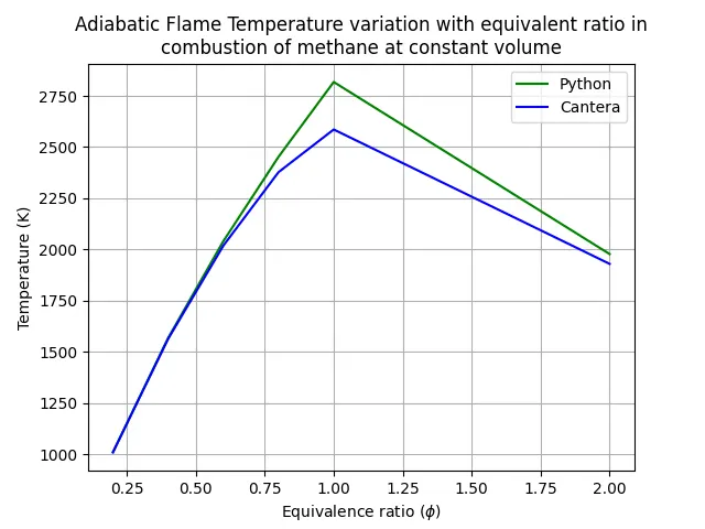
Now when we see the python code it does not include all the species involved in the combustion process but cantera takes into account all of the species. Hence the Cantera plot is said to be more accurate.
EFFECT OF AFT ON EQUIVALENCE RATIO WITH HEAT LOSS
import matplotlib.pyplot as plt
import math
import numpy as np


x = 1
y = 4
R = 8.314 #J/kmol-K
Qs = 802000	# As product are at gas phase Qs = LHV'mf = 50*e+6*16.04*e-3

H_loss = np.linspace(0,1,20)
H_product = []
H_reactants = []
def h(T, co_effs):

	R = 8.314 #J/mol-K
	al = co_effs[0]
	a2 = co_effs[1]
	a3 = co_effs[2]
	a4 = co_effs[3]
	a5 = co_effs[4]
	a6 = co_effs[5]

	return (al + a2*T/2 + a3*pow(T,2)/3 + a4*pow(T,3)/4 + a5*pow(T,4)/5 + a6/T)*R*T

ch4_coeffs_l	=	[5.14987613E+00,-1.36709788E-02,4.91800599E-05,-4.84743026E-08,1.66693956E-11,-1.02466476E+04,-4.64130376E+00]
o2_coeffs_l	=	[3.78245636E+00,-2.99673416E-03,9.84730201E-06,-9.68129509E-09,3.24372837E-12,-1.06394356E+03,3.65767573E+00]
n2_coeffs_l	=	[0.03298677E+02,0.14082404E-02,-0.03963222E-04,0.05641515E-07,-0.02444854E-10,-0.10208999E+04,0.03950372E+02]
n2_coeffs_h	=	[0.02926640E+02,0.14879768E-02,-0.05684760E-05,0.10097038E-09,-0.06753351E-13,-0.09227977E+04,0.05980528E+02]
co2_coeffs_h = [3.85746029E+00,4.41437026E-03,-2.21481404E-06,5.23490188E-10,-4.72084164E-14,-4.87591660E+04,2.27163806E+00]
h2o_coeffs_h = [3.03399249E+00,2.17691804E-03,-1.64072518E-07,-9.70419870E-11,1.68200992E-14,-3.00042971E+04,4.96677010E+00]
o2_coeffs_h	= [3.28253784E+00,1.48308754E-03,-7.57966669E-07,2.09470555E-10,-2.16717794E-14,-1.08845772E+03,5.45323129E+00]
co_coeffs_h = [2.71518561E+00,2.06252743E-03,-9.98825771E-07,2.30053008E-10,-2.03647716E-14,-1.41518724E+04,7.81868772E+00]

def f(T,H_loss):

	h_co2_p = h(T,co2_coeffs_h)
	h_h2o_p = h(T,h2o_coeffs_h)
	h_n2_p = h(T,n2_coeffs_h)
	H_product = h_co2_p + 2*h_h2o_p + 7.52*h_n2_p
	Tstd = 298.15
	h_ch4_r = h(Tstd,ch4_coeffs_l)
	h_o2_r = h(Tstd,o2_coeffs_l)
	h_n2_r = h(Tstd,n2_coeffs_l)
	H_reactants = h_ch4_r + 2*h_o2_r + 7.52*h_n2_r

	return H_product - H_reactants + (H_loss*Qs)

#	Newton Rapson Method to solve for AFT iteratively
def fprime(T,H_loss):
	return(f(T+1e-6,H_loss) - f(T,H_loss))/1e-6


#	Method solves for AFT till satisfying the criteria of tolerence
tol = 1e-3
alpha = 0.9
Temp=[]

#	Newton Rapson Method
for i in H_loss:
	T_guess = 1500
	R = 8.314 #J/mol-K

	while(abs(f(T_guess,i))> tol):
		T_guess = T_guess - alpha*((f(T_guess,i)/fprime(T_guess,i)))

	Temp. append(T_guess)

print(Temp)
T_loss = (Temp[10])
print(T_loss)

plt.figure(1)
plt.plot(H_loss,Temp, color = 'yellow')
plt.xlabel('H loss coefficient')
plt.ylabel('Adiabatic Flame Temperature')
plt.title('Effect of AFT on Equivalence Ratio with heat loss')
plt.grid()
plt.show()
This code takes into account of heat lossess. The above code is similar to the previos one, only this time H_loss parameter is added to the function to compute the reactions
PLOT FROM CODE
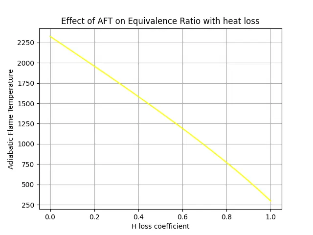
The AFT for the 1678.83 K for heat loss coefficient of 0.35. The variation of heat loss and Adiabatic flame temperature is linear. As the heat loss coefficient increases from 0 to 1, we can observe that there is minimum heat loss due to heat loss coefficient parameter.
FUEL SPECIES VERSUS AFT
import matplotlib.pyplot as plt
import numpy as np
import cantera as ct

gas = ct.Solution('gri30.xml')

gas.TPX = 298.15,101325,{'C2H2':1 ,'O2':3.5, 'N2':9.4}
gas.equilibrate('HP','auto')
T_c2h2 = gas.T

gas.TPX = 298.15,101325,{'C2H4':1, 'O2':3.5, 'N2':11.28}
gas.equilibrate('HP','auto')
T_c2h4 = gas.T

gas.TPX = 298.15,101325,{'C2H6':1, 'O2':3.5, 'N2':13.16}
gas.equilibrate('HP','auto')
T_c2h6 = gas.T

temp = (T_c2h2,T_c2h4,T_c2h6)
temp= np.array(temp)
print(temp)

plt.figure()
plt.bar(['C2H2','C2H4','C2H6'],temp, color = 'red')
plt.xlabel('Fuel Species')
plt.ylabel('Adiabatic Flame Temperature')
plt.title('AFT vs Fuel type(Cantera)')
plt.show()
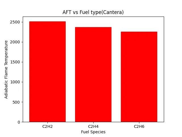
This small code was written in cantera to compute the adiabatic flame temperature for alkane, alkene and alkyne forms of hydrocarbons. First we call in the gas solving library, and then we define the basic froms of alkane, alkene and alkyne respectively. The gas.TPX command is used to define STP conditions at the beginning of the combustion process. The gas equilibrate command helps us to define which parameters should be calculated, in this case we are computing the enthalpies.
PLOT FOR FUEL SPECIES VERSUS AFT
EFFECT OF NUMBER OF CARBON ATOMS ON AFT
import matplotlib.pyplot as plt
import math
import numpy as np

def h(T,co_effs):

	R = 8.314 #J/mol-K
	al = co_effs[0]
	a2 = co_effs[1]
	a3 = co_effs[2]
	a4 = co_effs[3]
	a5 = co_effs[4]
	a6 = co_effs[5]

	return (al + a2*T/2 + a3*pow(T,2)/3 + a4*pow(T,3)/4 + a5*pow(T,4)/5 + a6/T)*R*T

ch4_coeffs_l = [5.14987613E+00,-1.36709788E-02,4.91800599E-05,-4.84743026E-08,1.66693956E-11,-1.02466476E+04,-4.64130376E+00]
c2h6_coeffs_l = [4.29142492E+00,-5.50154270E-03,5.99438288E-05,-7.08466285E-08,2.68685771E-11,-1.15222055E+04,2.66682316E+00]
c3h8_coeffs_l = [0.93355381E+00,0.26424579E-01,0.61059727E-05,-0.21977499E-07,0.95149253E-11,-0.13958520E+05,0.19201691E+02]
# Coefficients for Oxidiser: Oxygen(o2),Nitrogen(N2)
o2_coeffs_l = [3.78245636E+00,-2.99673416E-03,9.84730201E-06,-9.68129509E-09,3.24372837E-12,-1.06394356E+03,3.65767573E+00]
n2_coeffs_l = [0.03298677E+02,0.14082404E-02,-0.03963222E-04,0.05641515E-07,-0.02444854E-10,-0.10208999E+04,0.03950372E+02]
# Coefficients for Products at high temperature: Co2,H2o,N2
n2_coeffs_h = [0.02926640E+02,0.14879768E-02,-0.05684760E-05,0.10097038E-09,-0.06753351E-13,-0.09227977E+04,0.05980528E+02]
co2_coeffs_h = [3.85746029E+00,4.41437026E-03,-2.21481404E-06,5.23490188E-10,-4.72084164E-14,-4.87591660E+04,2.27163806E+00]
h2o_coeffs_h = [3.03399249E+00,2.17691804E-03,-1.64072518E-07,-9.70419870E-11,1.68200992E-14,-3.00042971E+04,4.96677010E+00]
Tstd = 298.15
H1 = h(Tstd,ch4_coeffs_l)
H2 = h(Tstd,c2h6_coeffs_l)
H3 = h(Tstd,c3h8_coeffs_l)
H = [H1,H2,H3]
H = np.array(H)
def f(T,H):

#Function that represent the root finding problem
	h_co2_p = h(T,co2_coeffs_h)
	h_h2o_p = h(T,h2o_coeffs_h)
	h_n2_p = h(T,n2_coeffs_h)
	h_o2_r = h(Tstd,o2_coeffs_l)
	h_n2_r = h(Tstd,n2_coeffs_l)

	if H == H1:
		x = 1
		y = 4
		a = x + (y/4)
		H_product = x*h_co2_p + (y/2)*h_h2o_p + (3.76*a)*h_n2_p
		H_reactants = H1 + a*h_o2_r + (3.76*a)*h_n2_r
	elif H == H2:
		x = 2
		y = 6
		a = x + (y/4)
		H_product = x*h_co2_p + (y/2)*h_h2o_p + (3.76*a)*h_n2_p
		H_reactants = H2 + a*h_o2_r + (3.76*a)*h_n2_r
	elif H == H3:
		x = 3
		y = 8
		a = x + (y/4)
		H_product = x*h_co2_p + (y/2)*h_h2o_p + (3.76*a)*h_n2_p
		H_reactants = H3 + a*h_o2_r + (3.76*a)*h_n2_r
	return H_product - H_reactants

def fprime(T,H):
	return(f(T+1e-6,H) - f(T,H))/1e-6

T_guess = 1500
tol = 1e-3
ct = 0
alpha = 0.9
temp = []

for i in H:
	R = 8.314 #J/mol-K
	while(abs(f(T_guess,i))> tol):
			T_guess = T_guess - alpha*((f(T_guess,i)/fprime(T_guess,i)))
	temp. append(T_guess)
plt.figure()
plt.bar(['CH4','C2H6','C3H8'],temp, color = 'green')
plt.ylabel('Adiabatic Flame Temperature')
plt.xlabel('Fuel Species')
plt.title('Effect of number of Carbon atoms')
plt.show()
PLOT OF NUMBER OF CARBON ATOMS VERSUS AFT
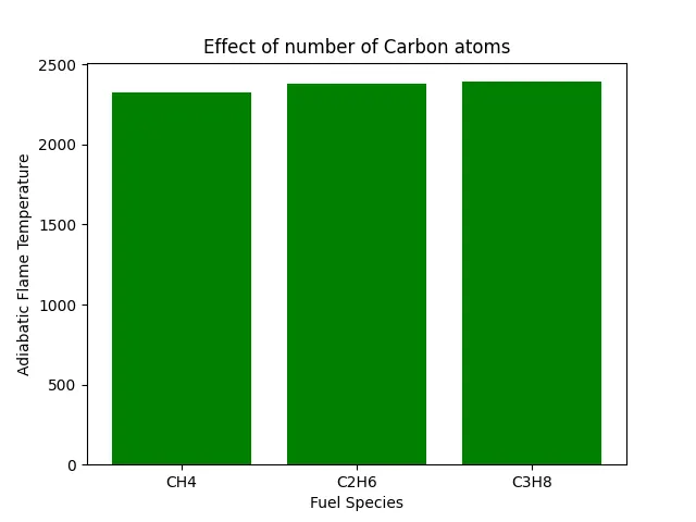
The information that was derived from the above plot is the AFT increases with number of Carbon atoms
CONCLUSION
- The effect of equivalence ratio was observed with AFT
- Other effects like heat loss, different fuel species and number of carbon atoms are also observed
- Comparison of Python and Cantera solvers were made which predicts the chemical reactions more accurately compared to python.