Week 3.5 - Deriving 4th order approximation of a 2nd order derivative using Taylor Table method
Deriving the fourth order approximation of a second order derivative :
Central difference method :
the taylor's approximation for a second order derivative is given as follows :
`(d^2u)/dx^2` `approx` `a*f(i) + b*f(i+1) + c*f(i+2) + d*f(i+3) + e*f(i+4) + g*f(i+5)`
here we have considered 5 nodes , according to the formula for central difference scheme; no. of nodes = p + q - 1
where, p = order of derivative; q = order of accuracy.
Note that we have multiplied co-efficients to the terms and we have to deduce them later.
Now we will expand the individual terms in taylor's approximation method,
`a*f(i-2) = a[f(i) - f'(i)*(2*dx)/(1!) + f''(i)*(2dx)^2/(2!) - f'''(i)(2dx)^3/(3!) + f^4(i)*(2dx)^4/(4!) - f^5(i)*(2dx)^5/(5!)]`
`b*f(i-1)` = `b[f(i) - f'(i)*dx/(1!) + f''(i)*(dx)^2/(2!) - f'''(i)(dx)^3/(3!) + f^4(i)*(dx^4)/(4!) - f^5(i)*(dx^5)/(5!)`
`c*f(i) = c*f(i)`
`d*f(i+1) = d[f(i) + f'(i)*(dx)/(1!) + f''(i)*(dx)^2/(2!) + f'''(i)*(dx)^3/(3!) + f^4(dx)^4/(4!) + f^5(i)*(dx^5)/(5!)]`
`e*f(i+2) = e[f(i) + f'(i)*(2dx)/(1!) + f''(i)(2dx)^2/(2!) + f'''(i)*(2dx^3)/(3!) + f^4(2dx^4)/(4!) + f^5(i)(2dx^5)/(5!)]`
Now we take the common derivative terms out and present it as follows :
`(d^2u)/(dx^2) approx [a + b + c + d + e]*f(i) + [-a*2*dx-b*dx+dx+2dx]*f'(i) +`
`[a*2*(dx^2) + b/2 * (dx)^2 + d*(dx^2)/2 + 2*d*(dx^2)]*f''(i)`
`+ [-a*8*(dx^3)/6 - b*(dx^3)/6 + d*(dx^3)/6 + d*8*(dx^3)/6]*f'''(i)`
`+ [a*16*(dx^4)/24+b*(dx^4)/24+d*(dx^4)/24+e*16*(dx^4)/24]*f^4(i)`
`+ [-a*32*(dx^5)/120-b*(dx^5)/120+d*(dx^5)/120+e*32*(dx^5)/120]*f^5(i)`
Now that we have manipulated the derivation in conceivable manner, we will represent it in a matrix form to calculate the coefficients a,b,c,d,e.
`[[1,1,1,1,1],[-2,-1,0,1,2],[2,1/2,0,1/2,2],[-8/6,-1/6,0,1/6,8/6],[16/24,1/24,0,1/24,16/24]]` * `[[a],[b],[c],[d],[e]]` = `[[0],[0],[1],[0],[0]]`
after deducing all the coefficients we utilize them in the derivation as follows :
`(d^2u)/(dx^2) approx -0.0833*f(i-2) + 1.3333*f(i-1) - 2.5000*f(i) + 1.3333*f(i+1) - 0.0833*f(i+2)`
Hence we have derived the expression for fourth order approximation of second order derivative using central difference method.
The Taylor's Table expansion for Left side skewed scheme for second order derivative if fourth order approximation is given as follows :
`(d^2u)/(dx^2) approx a*f(i-5) + b*f(i-4) + c*f(i-3) + d*f(i-2) + e*f(i-1) + g*f(i)`
and with similar manipulation to the central difference method, we get the following matrix :-
`[[1,1,1,1,1,1],[-5,-4,-3,-2,-1,0],[25/2,8,9/2,2,1/2,0],[-125/6,-64/6,-27/6,-8/6,-1/6,0],[625/24,256/24,81/24,16/24,1/24,0],[-3125/120,-1024/120,-243/120,-32/120,-1/120,0]]` `* [[a],[b],[c],[d],[e],[g]]``= [[0],[0],[1],[0],[0],[0]]`
again after solving this matrix we get the coefficients and the final expression is given as :
`(d^2u)/(dx^2) approx -8.333*f(i-5) + 5.0833*f(i-4)-13.000*f(i-3)+17.8333*f(i-2)-12.8333*f(i-1)+3.7500*f(i)`
Similarly for right skewed fourth order approximation of second order derivative is as follows :
the taylor's table expansion is :
`(d^2u)/(dx^2) approx a*f(i)+b*f(i+1)+c*f(i+2)+d*f(i+3)+e*f(i+4)+g*f(i+5)`
after similar manipulation of above cases ,the matrix for right skewed method is :
`[[1,1,1,1,1,1],[0,1,2,3,4,5],[0,1/2,2,9/2,8,25/2],[0,1/6,8/6,27/6,64/6,125/6],[0,1/24,16/24,81/24,256/24,625/24],[0,1/120,32/120,243/120,1024/120,3125/120]]` `* [[a],[b],[c],[d],[e],[g]] = [[0],[0],[1],[0],[0],[0]]`
Hence, the right sided skewed expression for this case is :
`(d^2u)/(dx^2) approx 3.7500*f(i) - 12.8333*f(i+1)+17.8333*f(i+2)-13*f(i+3)-5.0833*f(i+4)-0.8333*f(i+5)`
## Proof that these skewed schemes are fourth order accurate :
Usually we claim a taylor's table expansion as `n^(th)` order of approximation based on which order of term we are ignoring.
Here we have a formula: The order of accuracy P = Number of nodes in the stencil N - order of derivative Q (for one-sided/skewed schemes )
This way we can say that for left/right hand side skewed schemes for second order derivative require 6 number of nodes to be fourth order accurate. And in central difference method the formula becomes :
The order of accuracy P = Number of nodes in the stencil N - order of derivative Q + 1 (for symmetric/central schemes)
## Now we make a program in Matlab which will provide the graphical representation of how these 3 methods of approximation behaves with respect to the change in dx.
Here we consider the analytical function : exp(x)*cos(x)
the code is as follows :
clear all
close all
clc

% analytical derivative of exp(x)*cos(x)
% f''(x) = -2*exp(x)*sin(x)

x = pi/3;
dx = linspace(pi/400,pi/4,100);
analytical_second_derivative = -2*exp(x)*sin(x);

for i = 1:length(dx)

    central_error(i)  = fourth_central(x,dx(i));
    right_error(i) = fourth_approx_right(x,dx(i));
    left_error(i) = fourth_approx_left(x,dx(i));

end

figure(1)
loglog(dx,central_error,'color','b','linewidth',2)
hold on
loglog(dx,right_error,'color','r','linewidth',2)
hold on
loglog(dx,left_error,'color','g','linewidth',2)
legend('central difference error','right side skewed error','left side skewed error','Location','southeast')
xlabel('dx')
ylabel('error')
All three schemes are solved in separate functions and the values to the co-efficients are utilized directly from the matrix so as to avoid any error.
the functions are as follows :
central difference :
function out = fourth_central(x,dx)

% central

M = [1 1 1 1 1;
    -2 -1 0 1 2;
    2 1/2 0 1/2 2;
    -8/6 -1/6 0 1/6 8/6;
    16/24 1/24 0 1/24 16/24]

N = [0;0;1;0;0]

Z = inv(M)*N

% analytical second order derivative of exp(x)*cos(x)
% f''(x) = -2*exp(x)*sin(x)

analytical_second_derivative = -2*exp(x)*sin(x);

central_diff = (Z(1)*exp(x-2*dx)*cos(x-2*dx) + Z(2)*exp(x-dx)*cos(x-dx) + Z(3)*exp(x)*cos(x) + Z(4)*exp(x+dx)*cos(x+dx) + Z(5)*exp(x+2*dx)*cos(x+2*dx))/(dx^2)

out = abs(central_diff - analytical_second_derivative)

end
right side skewed scheme :
function out = fourth_approx_right(x,dx)

% right skewed
A = [ 1 1 1 1 1 1;
    0 1 2 3 4 5;
    0 1/2 2 9/2 8 25/2;
    0 1/6 8/6 27/6 64/6 125/6;
    0 1/24 16/24 81/24 256/24 625/24;
    0 1/120 32/120 243/120 1024/120 3125/120]


B = [0;0;1;0;0;0]

X = inv(A)*B


% analytical second order derivative of exp(x)*cos(x)
% f''(x) = -2*exp(x)*sin(x)

analytical_second_derivative = -2*exp(x)*sin(x);

right_skewed = (X(1)*exp(x)*cos(x) + X(2)*exp(x+dx)*cos(x+dx) + X(3)*exp(x+2*dx)*cos(x+2*dx) + X(4)*exp(x+3*dx)*cos(x+3*dx) + X(5)*exp(x+4*dx)*cos(x+4*dx) + X(6)*exp(x+5*dx)*cos(x+5*dx))/(dx^2)

out = abs(right_skewed-analytical_second_derivative)

end
left side skewed :
function out = fourth_approx_left(x,dx)

%  left skewed

C = [1 1 1 1 1 1;
    -5 -4 -3 -2 -1 0;
    25/2 8 9/2 2 1/2 0;
    -125/6 -64/6 -27/6 -8/6 -1/6 0;
    625/24 256/24 81/24 16/24 1/24 0;
    -3125/120 -1024/120 -243/120 -32/120 -1/120 0]


D = [0;0;1;0;0;0]

Y = inv(C)*D

% analytical second order derivative of exp(x)*cos(x)
% f''(x) = -2*exp(x)*sin(x)

analytical_second_derivative = -2*exp(x)*sin(x);

left_skewed = (Y(1)*(exp(x-5*dx)*cos(x-5*dx)) + Y(2)*(exp(x-4*dx)*cos(x-4*dx)) + Y(3)*(exp(x-3*dx)*cos(x-3*dx)) + Y(4)*(exp(x-2*dx)*cos(x-2*dx)) + Y(5)*exp(x-dx)*cos(x-dx) + Y(6)*(exp(x)*cos(x)))/(dx^2)

out = abs(left_skewed - analytical_second_derivative)

end
all the co-efficients are calculated in the respective functions.
the plot comparison for these methods is given as follows :
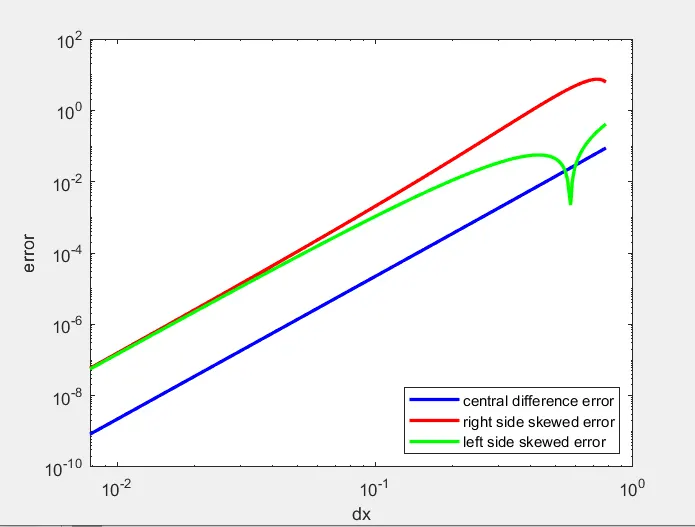
this plot compares the absolute error as difference between the analytical derivative and the approximated taylor's table expansion result for the particular method with respect to the value of dx.
As per the graph, we can see that the central difference is very much efficient in reducing the absolut error in comparison to the other skewed methods.
## why skewed schemes are used ,and what they can do which central difference method can't ?
skewed schemes are used when there are no equal no. of nodes available at both sides on a stencil. when the information taken from both sides is not symmetrical, skewed schemes are used and additional nodes are considered where we can. Mostly skewed schemes are used at the border surfaces where the geometry ends, there we are bound to use these schemes.
Central difference requires lesser number of nodes in comparison with the skewed schemes.
======================End=========================