Week 3.5 - Deriving 4th order approximation of a 2nd order derivative using Taylor Table method
Aim:-
Write a program for 4th order approximation of the second order derivative by using central difference, Skewed right-sided difference and Skewed left-sided difference by using taylor table method and to compare the exact derivative.
1] Central differencing scheme:-
given: P+Q = 1
where P = Order of derivative.
Q = Order of approximations.
P= 2 ; Q= 4
2+4=1
6-1=0
5
since no of nodes is 5
`d^2u/dx^2 = [a f(i-2)+ bf(i-1) +c f(i) +d f(i+1) + e f(1+2) ]/ dx^2` --------(A)`
`a f(i-2) = a f(i) - [ a f'(i) (2 dx) ] + [a f''(i) (2 dx)^2 ] / 2! - [a f ''' (i) (2 dx)^3]/3! + [ a f''''(i) (2 dx)^4] / 4!` -----(1)
Similarly we can solve for each term, for further values it's will be shown in the table with the help of taylor table method
| `dx^2 f''(i)` | f(i) | f'(i) `dx^2` |
f"(i) `dx^3` |
f"'(i) `dx^4` | f"''(i) `dx^5` |
| a f(i-2) | a | -2a | 2a | - 4a/3 | 2a/3 |
| b f(i-1) | b | b | b/2 | b/6 | b/24 |
| c f(i) | c | 0 | 0 | 0 | 0 |
| d f(i+1) | d | d | d/2 | d/6 | d/24 |
| e f(i+2) | e | 2e | 2e | 4e/3 | 2e/3 |
|
Sum of all co -efficient |
0 | 0 | 1 | 0 | 0 |
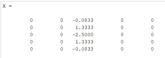
a+b+c+d+e=0
-2a+b+0+d+2e=0
2a+b/2+0+d/2+2e=1
-4/3 a+ b/6 +0+d/6+4/3e=0
2/3a + b/24 +0+d/24 +2/3e =0
2] Skewed right - sided scheme:
given: P+Q
where P = Order of derivative.
Q = Order of approximations.
P = 2 & Q = 4
P+Q= 4+2 = 6
since no of nodes is 6
`d^2u/dx^2 = [ a f(i) + b f(i+1) + c f(i+2) + d f(i+3) + e f(i+4) + g f(i+5) ] / dx^2` ---------(B)
Expanding all the terms shown in the equation B with the help of taylor table method
| `dx^2`f''(i) | f(i) | f'(i)dx | f''(i)`dx^2` | f'''(i) `dx^3` | f''''(i) `dx^4` | f'''''(i) `dx^5` |
| a f(i) | a | 0 | 0 | 0 | 0 | 0 |
| b f(i+1) | b | b | b/2 | b/6 | b/24 | b/120 |
| c f(i+2) | c | 2c | 2c | 4c/3 | 2c/3 | 32c/120 |
| d f(i+3) | d | 3d | 9d/2 | 27d/6 | 81d/24 | 243d/120 |
| e f(i+4) | e | 4e | 16e/2 | 64e/6 | 256e/24 | 1024e/120 |
| g f(i+5) | g | 5g | 25g/2 | 125g/6 | 625g/24 | 3125g/120 |
sum of all 0 0 1 0 0 0
co-efficient
equations,
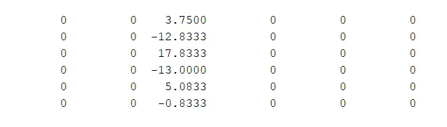
a+b+c+d+e+g=0
0+b+2c+3d+4e+5g=0
0+b/2+2c+9d/2+16e/2+25g/2=1
0+b/6+4c/3+27d/6+64e/6+125g/6=0
0+b/24+2c/3+81d/24+256e/24+625g/24=0
0+b/120+32c/120+24d/120+1024e/120+3125g/120=0
3] Skewed left - sided scheme:
given: P+Q
where P = Order of derivative.
Q = Order of approximations.
P = 2 & Q = 4
P+Q= 4+2 = 6
since no of nodes is 6 from the left side.
`d^2u/dx^2=[a f(i-5) +b f(i-4) + c f(i-3) + d f(i-2) +e f(i-1) + g f(i) ] / dx^2` -------- (C`
`a f(i-5) = a f(i) - a f'(i)(5 dx) / 1! + a f''(i)(5 dx)^2 / 2! - a f'''(i)(5 dx)^3 / 3! + a f''''(i)(5 dx)^4 / 4! -a f''"'''(i)(5 dx)^5 / 5!`
Expanding all the terms shown in the equation B with the help of taylor table method
| f(i) | f'(i) dx | f"(i) dx^2 | f"'(i) dx^3 | f''''(i) dx^4 | f""'(i) dx^5 | |
| f(i-5) | a | -5a | 25a/2 | -125a/6 | 625a/24 | -3125a/120 |
| f(i-4) | b | -4b | 16b/2 | -64b/6 | 256b/24 | -1024b/120 |
| f(i-3) | c | -3c | 9 c /2 | -27c/6 | 81c/24 | -243c/120 |
| f(i-2) | d | -2d | 4d / 2 | -8d/6 | 16d/24 | -32d/120 |
| f(i-1) | e | -e | e / 2 | -e/6 | e/24 | -e/120 |
| f(i) | g | 0 | 0 | 0 | 0 | 0 |
Sum all of the 0 0 1 0 0 0
co-efficient
Equations,
a+b+c+d+e+g=0
-5a-4b-3c-2d-e+0=0
25a/2+16b/2+9c/2+4d/2+e/2+0=1
-125a/6-64b/6-27c/6-8d/6-e/6+0=0
625a/24+256b/24+81c/24+16d/24+e/24+0=0
-3125a/120-1024b/120-243c/120-32d/120-e/120-0=0
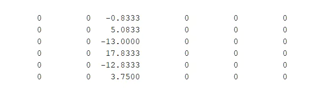
where a= -0.8333
b= 5.0833
c= -13.0000
d= 17.8333
e= -12.8333
g= 3.7500
Main code:-
clear all
close all
clc

% value of x
x= pi/3 ;

% Value of dx
dx= linspace(pi/4,pi/4000,20);

for i=1:length(dx)
central_differencing(i)=error_central_differencing_approximation(x,dx(i));
 skewed_right_hand(i)= error_skewed_right_hand_approximation(x,dx(i));
 skewed_left_hand(i)=error_skewed_left_hand_approximation(x,dx(i));
end

%plotting

figure(1)
loglog(dx,central_differencing,'r','LineWidth',3)
hold on
loglog(dx,skewed_right_hand,'g','LineWidth',3)
hold on
loglog(dx,skewed_left_hand,'b','LineWidth',3)
xlabel('range of dx')
ylabel('truncation error')
title('range of dx vs error')
legend('central differencing','skewed right sided difference','skewed left sided difference','location','northwest')
function error_central_differencing-
function error_central_differencing= error_central_differencing_approximation(x,dx)

% analytical function = exp(x)*cos(x)
% f'(x) = -exp(x)*sin(x)+cos(x)*exp(x)
% f''(x) = exp(x)[cos(x)-sin(x)]
% f''(x) = exp(x)[-sin(x)-cos(x)+ exp(x)[cos(x)-sin(x)]
% f''(x) = -exp(x)*sin(x)-exp(x)*cos(x)+exp(x)*cos(x)-exp(x)*sin(x)
% f''(x) = -2*exp(x)*sin(x)

% Analytical function for second order
Analytical_function  = -2*exp(x)*sin(x) ;

% Central differencing
% d^2u/dx^2 = [a f(i-2)+ bf(i-1) +c f(i) +d f(i+1) + e f(1+2) ]/ dx^2 ;

a= [1 1 1 1 1 ; -2 -1 0 1 2 ; 2 1/2 0 1/2 2 ; -4/3 -1/6 0 1/6 4/3 ; 2/3 1/24 0 1/24 2/3 ]

b= [ 0; 0; 1; 0; 0 ]

[C]= inv(a)*b

% central_differencing = (-0.0833*exp(x-2*dx)*cos(x-2*dx)+1.3333*exp(x-dx)*cos(x-dx)-2.5000*exp(x)*cos(x)+1.3333*exp(x+dx)*cos(x+dx)-0.0833*exp(x+2*dx)*cos(x+2*dx))/(dx^2) ;
central_differencing =(C(1)*exp(x-2*dx)*cos(x-2*dx)+C(2)*exp(x-dx)*cos(x-dx)+C(3)*exp(x)*cos(x)+C(4)*exp(x+dx)*cos(x+dx)+C(5)*exp(x+2*dx)*cos(x+2*dx))/(dx^2) ;

error_central_differencing= abs(central_differencing-Analytical_function);

end
function error_skewed_right_hand:-
function error_skewed_right_hand = error_skewed_right_hand_approximation(x,dx)

% analytical function = exp(x)*cos(x)
% f'(x) = -exp(x)*sin(x)+cos(x)*exp(x)
% f''(x) = -2*exp(x)*sin(x)

% Analytical function for second order
Analytical_function  = -2*exp(x)*sin(x) ;

% skewed_right_hand
 % d^2u/dx^2 = [ a f(i) + b f(i+1) + c f(i+2) + d f(i+3) + e f(i+4) + g f(i+5) ] / dx^2

a=[ 1 1 1 1 1 1 ; 0 1 2 3 4 5 ; 0 1/2 2 9/2 16/2 25/2 ; 0 1/6 4/3 27/6 64/6 125/6 ; 0 1/24 2/3 81/24 256/24 625/24 ; 0  1/120 32/120 243/120 1024/120 3125/120 ]

b = [ 0; 0; 1; 0; 0; 0 ]

[C]=inv(a)*b

% skewed_right_hand =(3.7500*exp(x)*cos(x)-12.8333*exp(x+dx)*cos(x+dx)+17.8333*exp(x+2*dx)*cos(x+2*dx)-13.0000*exp(x+3*dx)*cos(x+3*dx)+5.0833*exp(x+4*dx)*cos(x+4*dx)-0.8333*exp(x+5*dx)*cos(x+5*dx))/(dx^2);
skewed_right_hand =(C(1)*exp(x)*cos(x)+C(2)*exp(x+dx)*cos(x+dx)+C(3)*exp(x+2*dx)*cos(x+2*dx)+C(4)*exp(x+3*dx)*cos(x+3*dx)+C(5)*exp(x+4*dx)*cos(x+4*dx)+C(6)*exp(x+5*dx)*cos(x+5*dx))/(dx^2)
error_skewed_right_hand=abs(skewed_right_hand-Analytical_function);

end
function error_skewed_left_hand:-
function error_skewed_left_hand = error_skewed_left_hand_approximation(x,dx)

% analytical function = exp(x)*cos(x)
% f'(x) = -exp(x)*sin(x)+cos(x)*exp(x)
% f''(x) = -2*exp(x)*sin(x)

% Analytical function for second order
Analytical_function  = -2*exp(x)*sin(x) ;

% skewed_left_hand

% d^2u/dx^2=[a f(i-5) + b f(i-4) + c f(i-3) + d f(i-2) + e f(i-1) + g f(i)] / dx^2


a=[ 1 1 1 1 1 1 ; -5 -4 -3 -2 -1 0 ; 25/2 16/2 9/2 2 1/2 0 ;-125/6 -64/6 -27/6 -8/6 -1/6 0 ; 625/24 256/24 81/24 16/24 1/24 0; -3125/120 -1024/120 -243/120 -32/120 -1/120 0]

b=[0;0 ;1; 0; 0; 0 ]

[C]=inv(a)*b


% skewed_left_hand=(-0.8333*exp(x-5*dx)*cos(x-5*dx)+5.0833*exp(x-4*dx)*cos(x-4*dx)-13.0000*exp(x-3*dx)*cos(x-3*dx)+17.8333*exp(x-2*dx)*cos(x-2*dx)-12.8333*exp(x-1*dx)*cos(x-1*dx)+3.7500*exp(x)*cos(x))\(dx^2);
skewed_left_hand=(C(1)*exp(x-5*dx)*cos(x-5*dx)+C(2)*exp(x-4*dx)*cos(x-4*dx)+C(3)*exp(x-3*dx)*cos(x-3*dx)+C(4)*exp(x-2*dx)*cos(x-2*dx)+C(5)*exp(x-1*dx)*cos(x-1*dx)+C(6)*exp(x)*cos(x))/(dx^2)
error_skewed_left_hand=abs(skewed_left_hand-Analytical_function);

end
Plot:-
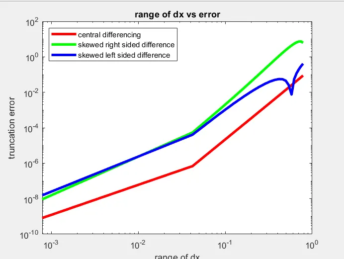
Conclusion:- As central differencing has less error as compared to skewed left & right side.