Objective:
To derive the following 4th order approximation of the second order derivative using
- Central difference
- Skewed rigth-sided difference
- Skewed left-sided difference
First step is to find the number of nodes required for deriving each difference method using the given formula.
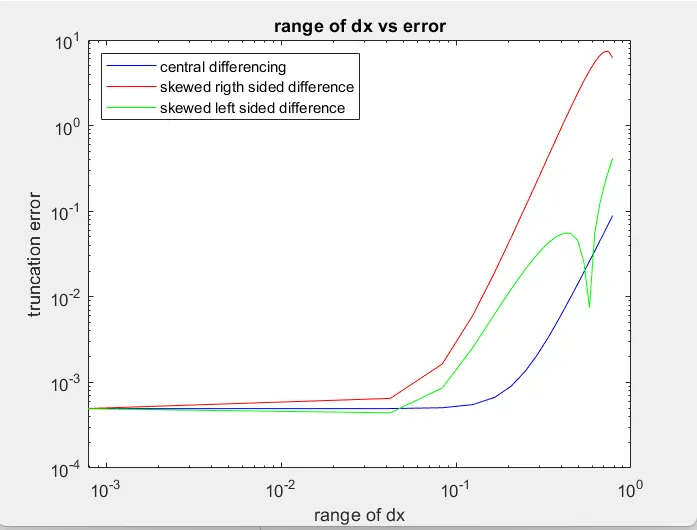
After deriving all the difference method, the other step is to compare all the derived difference method with the exact solution and to find the range of error for each difference method using MATLAB.
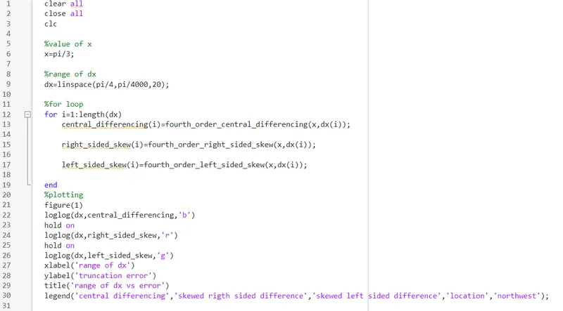
Main code
clear all
close all
clc
%value of x
x=pi/3;
%range of dx
dx=linspace(pi/4,pi/4000,20);
%for loop
for i=1:length(dx)
central_differencing(i)=fourth_order_central_differencing(x,dx(i));
right_sided_skew(i)=fourth_order_right_sided_skew(x,dx(i));
left_sided_skew(i)=fourth_order_left_sided_skew(x,dx(i));
end
%plotting
figure(1)
loglog(dx,central_differencing,'b')
hold on
loglog(dx,right_sided_skew,'r')
hold on
loglog(dx,left_sided_skew,'g')
xlabel('range of dx')
ylabel('truncation error')
title('range of dx vs error')
legend('central differencing','skewed rigth sided difference','skewed left sided difference','location','northwest');
central differencing function code
function Error_central_differencing = fourth_order_central_differencing(x,dx);
%analytic function = exp(x)*cos(x)
%analytical derivative
%f''(x)=-2*exp(x)sin(x)
analytical_derivative=-2*exp(x)*sin(x);
%numerical derivative
%central differencing
central_differencing=(((-0.0833)*((exp(x-(2*dx)))*(cos(x-(2*dx)))))+((1.3333)*((exp(x-dx))*((cos(x-dx))))-((2.5000)*((exp(x))*(cos(x))))+((1.3333)*((exp(x+dx))*(cos(x+dx))))-((0.0833)*((exp(x+(2*dx)))*cos(x+(2*dx))))))/(dx^2);
Error_central_differencing=abs(central_differencing-analytical_derivative);
right sided skew difference function code
function Error_right_sided_skew = fourth_order_right_sided_skew(x,dx);
%analytic function = exp(x)*cos(x)
%analytical derivative
%f''(x)=-2*exp(x)sin(x)
analytical_derivative=-2*exp(x)*sin(x);
%numerical derivative
%right sided skew
right_sided_skew=(((3.7500)*((exp(x))*(cos(x))))-((12.8333)*((exp(x+dx))*(cos(x+dx))))+((17.8333)*((exp(x+(2*dx)))*(cos(x+(2*dx)))))-((13.0000)*((exp(x+(3*dx)))*(cos(x+(3*dx)))))+((5.0833)*((exp(x+(4*dx)))*(cos(x+(4*dx)))))-((0.8333)*((exp(x+(5*dx)))*(cos(x+(5*dx))))))/(dx^2);
Error_right_sided_skew=abs(right_sided_skew-analytical_derivative);
end
left sided skew difference function code
function Error_left_sided_skew = fourth_order_left_sided_skew(x,dx);
%analytic function = exp(x)*cos(x)
%analytical derivative
%f''(x)=-2*exp(x)sin(x)
analytical_derivative=-2*exp(x)*sin(x);
%numerical derivative
%Left sided skew
left_sided_skew=(((-0.8333)*((exp(x-(5*dx)))*(cos(x-(5*dx)))))+((5.0833)*((exp(x-(4*dx)))*(cos(x-(4*dx)))))-((13.0000)*((exp(x-(3*dx)))*(cos(x-(3*dx)))))+((17.8333)*((exp(x-(2*dx)))*(cos(x-(2*dx)))))-((12.8333)*((exp(x-dx))*(cos(x-dx))))+((3.7500)*((exp(x))*(cos(x)))))/(dx^2);
Error_left_sided_skew=abs(left_sided_skew-analytical_derivative);
end
Output graph
Conclusion:
As seen from the plot the central differenceing scheme has very less error when compared to the other schemes. Therefore, central differencing scheme is better than other schemes because it uses information from both the sides from the point of consideration to give appropriate and accurate values.
As the left and right skewed difference methods uses data only from one side of point of interest it gives less approximation and accurate values about that point.
The system which doesn't contain sufficient information on both the side of the point of interest in such cases we cannot use central differencing scheme so skewed scheme is useful in such cases.