Week 3.5 - Deriving 4th order approximation of a 2nd order derivative using Taylor Table method

Aim:- Deriving 4th order approximation of a 2nd order derivative using Taylor Table method

Objective :-

Derive the following 4th order approximations of the second-order derivative.

1. Central difference

2. Skewed right-sided difference

3. Skewed left-sided difference

write a program in Matlab to evaluate the second-order derivative of the analytical function exp(x)*cos(x) and compare it with the 3 numerical approximations

Theory :-

Using Taylor series expansion, 4th order approximation of 2nd order derivative will be calculated using different schemes and these schemes are explained below

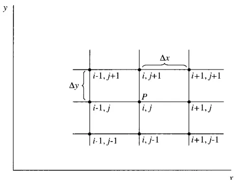
In the above figure, point P value can be calculated by three ways 1) using values from right side points 2) from left side points and 3) and by using both left and right side points

Due to using different sides , it is called right side difference , left side difference and central difference schemes

And for different order of approximations, lets take examples from below figure

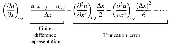
Above figure is first order derivative where finite difference and truncation error is given , order of approximation is indicated by the lowest degree of first `Deltax` in truncation error.

So, here for 4th order approximation lowest degree of `Deltax`in truncation error should be 4.

Using given HINTS , number of nodes in the stensil for different schemes can be calculated and it is found that for right and left side scheme, number of nodes will be 6 and for central scheme nodes will be 5.

The Hypothesis equation for all the schemes are:-

Right side difference

`(del^2f)/(delx^2) = (af(i) +bf(i+1)+cf(i+2)+df(i+3)+ef(i+4)+gf(i+5))/(Deltax^2)-O(Deltax)^4`

There are 6 unkowns in the above equation,so there should be 6 equations to be solved so taylor series expansion for each stensils will upto 5th derivative and is given below in Taylor table.

In the table the sum of all coefficients of each derivatives of all stensils will be 0 except 2nd derivative, instead it will have sum 1 because here we need to find approximation for 2nd derivative only if it also becomes 0 then 2nd derivative will not exist and this follows in all schemes.

Taylor table:-

	f(i)	`Deltaxf'(i)`	`(Deltax)^2f''(i)`	`(Deltax)^3f'''(i)`	`(Deltax)^4f^(iv) (i)`	`(Deltax)^5f^(v) (i)`
af(i)	a	0	0	0	0	0
bf(i+1)	b	b	`b/2`	`b/6`	`b/24`	`b/120`
cf(i+2)	c	2c	`(4c)/2`	`(8c)/6`	`(16c)/24`	`(32c)/120`
df(i+3)	d	3d	`(9d)/2`	`(27d)/6`	`(81d)/24`	`(243d)/120`
ef(i+4)	e	4e	`(16e)/2`	`(64e)/6`	`(256e)/24`	`(1024e)/120`
gf(i+5)	g	5g	`(25g)/2`	`(125g)/6`	`(625g)/24`	`(3125g)/120`
SUM =	0	0	1	0	0	0

Above coefficients can be calculated by

`a+b+c+d+e+g=0`

`0+b+2c+3d+4e+5g=0`

`0+b/2+(4c)/2+(9d)/2+(16e)/2+(25g)/2=1`

`0+b/6+(8c)/6+(27d)/6+(64e)/6+(125g)/6=0`

`0+b/24+(16c)/24+(81d)/24+(256e)/24+(625g)/24=0`

`0+b/120+(32c)/120+(243d)/120+(1024e)/120+(3125g)/120=0`

Writing above equations in the matrix form:-

`[[1,1,1,1,1,1],[0,1,2,3,4,5],[0,1,4,9,16,25],[0,1,8,27,64,125],[0,1,16,81,256,625],[0,1,32,243,1024,3125]] [(a),(b),(c),(d),(e),(g)]=[(0),(0),(2),(0),(0),(0)]`

After calculation, coefficient values are:-

a=3.7500

b=-12.8333

c=17.8333

d=-13.0000

e=5.0833

g=-0.8333

Left side difference

`(del^2f)/(delx^2) = (af(i) +bf(i-1)+cf(i-2)+df(i-3)+ef(i-4)+gf(i-5))/(Deltax^2)-O(Deltax)^4`

Taylor table:-

	f(i)	`Deltaxf'(i)`	`(Deltax)^2f''(i)`	`(Deltax)^3f'''(i)`	`(Deltax)^4f^(iv) (i)`	`(Deltax)^5f^(v) (i)`
af(i)	a	0	0	0	0	0
bf(i-1)	b	-b	`b/2`	`-b/6`	`b/24`	`-b/120`
cf(i-2)	c	-2c	`(4c)/2`	`-(8c)/6`	`(16c)/24`	`-(32c)/120`
df(i-3)	d	-3d	`(9d)/2`	`-(27d)/6`	`(81d)/24`	`-(243d)/120`
ef(i-4)	e	-4e	`(16e)/2`	`-(64e)/6`	`(256e)/24`	`-(1024e)/120`
gf(i-5)	g	-5g	`(25g)/2`	`-(125g)/6`	`(625g)/24`	`-(3125g)/120`
SUM =	0	0	1	0	0	0

Above coefficients can be calculated by

`a+b+c+d+e+g=0`

`0-b-2c-3d-4e-5g=0`

`0+b/2+(4c)/2+(9d)/2+(16e)/2+(25g)/2=1`

`0-b/6-(8c)/6-(27d)/6-(64e)/6-(125g)/6=0`

`0+b/24+(16c)/24+(81d)/24+(256e)/24+(625g)/24=0`

`0-b/120-(32c)/120-(243d)/120-(1024e)/120-(3125g)/120=0`

Writing above equations in the matrix form:-

`[[1,1,1,1,1,1],[0,-1,-2,-3,-4,-5],[0,1,4,9,16,25],[0,-1,-8,-27,-64,-125],[0,1,16,81,256,625],[0,-1,-32,-243,-1024,-3125]] [(a),(b),(c),(d),(e),(g)]=[(0),(0),(2),(0),(0),(0)]`

After calculation, coefficient values are:-

a=3.7500

b=-12.8333

c=17.8333

d=-13.0000

e=5.0833

g=-0.8333

Central difference schemes

`(del^2f)/(delx^2) = (af(i-2) -bf(i-1)+cf(i)-df(i+1)+ef(i+2))/(Deltax^2)-O(Deltax)^4`

Taylor table:-

	f(i)	`Deltaxf'(i)`	`(Deltax)^2f''(i)`	`(Deltax)^3f'''(i)`	`(Deltax)^4f^(iv) (i)`	`(Deltax)^5f^(v) (i)`
af(i-2)	a	-2a	`(4a)/2`	`(-8a)/6`	`(16a)/24`	`(-32a)/120`
bf(i-1)	b	-b	`b/2`	`-b/6`	`b/24`	`-b/120`
cf(i)	c	0	0	0	0	0
df(i+1)	d	d	`(d)/2`	`(d)/6`	`(d)/24`	`(d)/120`
ef(i+2)	e	2e	`(4e)/2`	`(8e)/6`	`(16e)/24`	`(32e)/120`
SUM =	0	0	1	0	0	?

Above coefficients can be calculated by

`a+b+c+d+e+g=0`

`-2a-b+0+d+2e=0`

`(4a)/2+b/2+0+(d)/2+(4e)/2=1`

`(-8a)/6-b/6+0+(d)/6+(8e)/6=0`

`(16a)/24+b/24+0+(d)/24+(16e)/24=0`

Writing above equations in the matrix form:-

`[[1,1,1,1,1],[-2,-1,0,1,2],[4,1,0,1,4],[-8,-1,0,1,8],[16,1,0,1,16]] [(a),(b),(c),(d),(e)]=[(0),(0),(2),(0),(0)]`

After calculation, coefficient values are:-

a= -0.0833

b= 1.3333

c = -2.5000

d = 1.3333

e = -0.0833

In the above coefficients we can see that

a = e and

b = d

so sum of coefficients of 5th derivative in central difference scheme will also be 0

MATLAB CODE:-

clear all
close all 
clc

% function is f(x)=exp(x)*cos(x)
%Let second derivative of f(x) at
x=pi/3;
%step size which is in range of
dx = linspace(pi/4,pi/4000,20);

for i=1:length(dx)
[error_right_side(i),right_side_second_derivative(i)] = right_side_difference(x,dx(i));
[error_left_side(i),right_side_second_derivative(i)] = left_side_difference(x,dx(i));
[error_center(i),center_side_second_derivative(i)] = center_difference(x,dx(i));
end

% plot
figure(1)
loglog(dx,error_right_side,'b')
hold on
loglog(dx,error_left_side,'r')
hold on
loglog(dx,error_center,'g')
hold off
xlabel('dx')
ylabel('error')
legend('Right side scheme','Left side scheme','central scheme','location','northwest')

Explanation:-

In the above code initial value of x is chosen as `pi/3` and step size which is in range of dx as `[pi/4 to pi/4000]` then for loop is used where functions of all different schemes has been called (details of these functions is given below) and error is calculated for all value of dx.

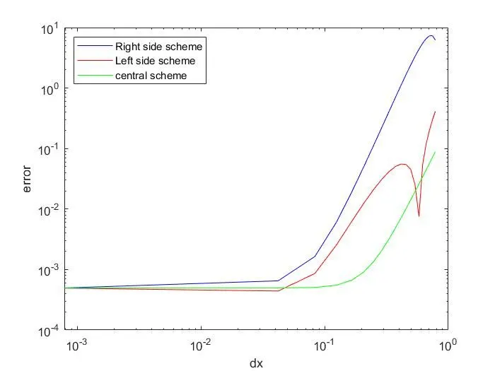
after having all the error value calculated from functions of different schemes a graph is plotted where x-axis denotes different value of dx and y-axis denotes errors. Here, blue curve is for right side scheme , red curve is for left side scheme and green curve is for central scheme.

Function for Right side difference scheme

function [error_right_side,right_side_second_derivative] = right_side_difference(x,dx)

%Analytical second order derivative of f(x)
analytical_derivative = (-2*(exp(x))*sin(x));
%Coefficient of right side difference
a=3.7500;
b=-12.8333;
c=17.8333;
d=-13.0000;
e=5.0833;
g=-0.8333;

%Stencils
A = exp(x)*cos(x);
B = exp(x+dx)*cos(x+dx);
C = exp(x+2*dx)*cos(x+2*dx);
D = exp(x+3*dx)*cos(x+3*dx);
E = exp(x+4*dx)*cos(x+4*dx);
G = exp(x+5*dx)*cos(x+5*dx);

%fourth order approximation 
right_side_second_derivative = ((a*A)+(b*B)+(c*C)+(d*D)+(e*E)+(g*G))/(dx^2);

error_right_side = abs(right_side_second_derivative-analytical_derivative);
end

EXPLANATION:-

The above code is function for right side difference where second derivative of the function is calculated by analytical and numerical descretization, here to reduce the length of formula in fourth order approximation all the stencil expressions are denoted by A,B,C,D,E,G. And coefficients which was calculated using taylor table is given by a,b,c,d,e,g, these coefficient values are used to find the derivative of the function.

After having value of second derivative of function by both methods their error is calculated by subtracting both values and their absolute error value found out.

Function for left side difference scheme

function [error_left_side,right_side_second_derivative] = left_side_difference(x,dx)

%Analytical second order derivative of f(x)
analytical_derivative = (-2*(exp(x))*sin(x));
%Coefficient of left side difference
m=3.7500;
n=-12.8333;
o=17.8333;
p=-13.0000;
q=5.0833;
r=-0.8333;

%Stencils
M = exp(x)*cos(x);
N = exp(x-dx)*cos(x-dx);
O = exp(x-2*dx)*cos(x-2*dx);
P = exp(x-3*dx)*cos(x-3*dx);
Q = exp(x-4*dx)*cos(x-4*dx);
R = exp(x-5*dx)*cos(x-5*dx);

%fourth order approximation 
right_side_second_derivative = ((m*M)+(n*N)+(o*O)+(p*P)+(q*Q)+(r*R))/(dx^2);

error_left_side = abs(right_side_second_derivative-analytical_derivative);
end

EXPLANATION:-

The above code is function for left side difference where second derivative of the function is calculated by analytical and numerical descretization, here to reduce the length of formula in fourth order approximation all the stencil expressions are denoted by M,N,O,P,Q,R. And coefficients which was calculated using taylor table is given by m,n,o,p,q,r, these coefficient values are used to find the derivative of the function.

After having value of second derivative of function by both methods their error is calculated by subtracting both values and their absolute error value found out.

Function for central difference scheme

function [error_center,center_side_second_derivative] = center_difference(x,dx)

%Analytical second order derivative of f(x)
analytical_derivative = (-2*(exp(x))*sin(x));
%Coefficient of central difference
u=-0.0833;
v=1.3333;
w=-2.5000;
y=1.3333;
z=-0.0833;

%Stencils
U = exp(x-2*dx)*cos(x-2*dx);
V = exp(x-dx)*cos(x-dx);
W = exp(x)*cos(x);
Y = exp(x+dx)*cos(x+dx);
Z = exp(x+2*dx)*cos(x+2*dx);

%fourth order approximation 
center_side_second_derivative = ((u*U)+(v*V)+(w*W)+(y*Y)+(z*Z))/(dx^2);

error_center = abs(center_side_second_derivative-analytical_derivative);
end

EXPLANATION :-

The above code is function for central difference where second derivative of the function is calculated by analytical and numerical descretization, here to reduce the length of formula in fourth order approximation all the stencil expressions are denoted by U,V,W,Y,Z. And coefficients which was calculated using taylor table is given by u,v,w,y,z, these coefficient values are used to find the derivative of the function.

After having value of second derivative of function by both methods, their error is calculated by subtracting both values and their absolute error value found out.

Conclusion:-

Second order derivative of function is derived here for fourth order approximation using different schemes which is skewed right side difference , skewed left side difference and central difference , all these schemes are derived using Taylor series expansion where different stencils are expanded tabulating them . Through this we got understanding of taylor table that how to construct it and how to use it . Order of approximation is identified by the lowest degree of dx in truncation error while expanding in taylor series expansion.

Coefficients of each term is calculated using MATLAB by arranging them in a equation and in matrix form which is shown above. Then different functions is written in matlab for different schemes where analytical derivative and numerical derivative of given function which is exp(x)*Cos(X) is calculated also their error is found out by subtracting both derivative values.

All the functions is called in main code where input x and range of dx is used for calculation and their graph is plotted using loglog command where it is found that central scheme is giving least error as compared by other schemes then by left scheme and maximum error is from right side scheme also at certain value of dx error is not so large but after that we can see slopes of all schemes increased rapidly from that we can say that as dx value is decreasing there is more chance of increase in error.

But using skewed scemes is more advantageous than central scheme and it depends upon different cases because if we take case of boundary condition then at boundary using central scheme will give incorrect result because central scheme uses values from both sides i.e., right and left nodes to calculate value at current position and boundaries have only one side so using skewed scheme at boundary will give accurate result.