Week 3.5 - Deriving 4th order approximation of a 2nd order derivative using Taylor Table method

WEEK 3.5 CHALLENGE:DETAILED REVIEW

OBJECTIVES:

Derive the following 4th order approximations of the second-order derivative.

1. Central difference

2. Skewed right-sided difference

3. Skewed left-sided difference

After deriving these schemes, prove that your skewed schemes are fourth-order accurate.

1)Central Difference:

i) The order of accuracy P = Number of nodes in the stencil N - order of derivative Q + 1 for symmetric/central schemes

Therefore Number of nodes in the stencil N = Order of accuracy (P) + Order of derivative(Q)-1

ie N=4+2-1=5

`((partial)^2*y)/((partial(x)^2)`= a.f(i-2)+b.f(i-1)+c.f(i)+d.f(i+1)+e.f(i+2)`

Then we need to expand each term by using Taylor-series method

`f(i-2)=a*[f(i)-f'(i).dx/1!`+f"(i).(dx)^2/2!-f"'(i).(dx)^3/3!+f""(i).(dx)^4/4!-f""'(i).(dx)^5/5!]`

`imiliarly we can expand each terms in that expression byen by writing the coefficients we will get Taylor-table

`((partial)^2f)/((partial(x))^2`	f(i)	f'(i).(dx)	f"(i).(dx)^2	f"'(i).(dx)^3	f""(i).(dx)^4	f""'(i).(dx)^5
a.f(i-2)	a	-2a	4a/2	-8a/6	16a/24	-32a/120
b.f(i-1)	b	-b	b/2	-b/6	b/24	-b/120
c.f(i)	c	0	0	0	0	0
d.(f(i+1)	d	d	d/2	d/6	d/24	d/120
e.f(i+2)	e	2e	4e/2	8e/6	16e/24	32e/120
Sum of coefficient	0	0	1	0	0	0

Here there are 5 unknowns and 5 equations are there and that 5 equations are given below:

a+b+c+d+e = 0 .................................(1)

-2a+(-b)+0+d+2e = 0.........................(2)

4a/2+b/2+0+d/2+4e/2 =1...................(3)

-8a/6+-b/6+0+d/6+8e/6 = 0...............(4)

16a/24+b/24+0+d/24+16e/24=0.........(5)

This system of equations we can solve by using matrix inversion method

therefore A=`[[1,1,1,1,1],[-2,-1,0,1,2],[4/2,1/2,0,1,2],[-8/6,-1/6,0,1/6,8/6],[16/24,1/24,0,1/24,16/24]]`

X=`[[a],[b],[c],[d],[e]]`

and B= `[[0],[0],[1],[0],[0]]`

So X=Inverse of A*B

After solving that matrix by using MATLAB we will get the value for unkonwn coefficients as given below:

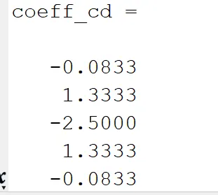
ie a= -0.0833, b=1.3333, c= -2.5000, d=1.3333 and e=-0.8333

ie a=e and b=d

Then substitute these values for f"'"(i).(dx)^5 and then we will sum as zero.

Divide f^6(i).(dx)^6/dx^2 then we will get the coefficient in the order of dx^4 so that we can say that this is 4th order approximation.

2. Skewed right-sided difference

The order of accuracy P = Number of nodes in the stencil N - order of derivative Q for one-sided/skewed schemes

So that N=P+Q = 4+2=6

`((partial)^2*y)/((partial(x)^2)`= a.f(i)+b.f(i+1)+c.f(i+2)+d.f(i+3)+e.f(i+4)+g.f(i+5)`

then we can create Taylor table by expandig each terms by Taylor series

`((partial)^2f)/((partial(x))^2`	f(i)	f'(i).(dx)	f"(i).(dx)^2	f"'(i).(dx)^3	f""(i).(dx)^4	f""'(i).(dx)^5
a.f(i)	a	0	0	0	0	0
b.f(i+1)	b	b	b/2	b/6	b/24	b/120
c.f(i+2)	c	2c	4c/2	8c/6	16c/24	32c/120
d.(f(i+3)	d	3d	9d/2	27d/6	81d/24	243d/120
e.f(i+4)	e	4e	16e/2	64e/6	256e/24	1024e/120
g.f(i+5)	g	5g	25g/2	125g/6	625g/24	3125g/120
Sum of coefficient	0	0	1	0	0	0

Here we have 6 unknowns(a,b,c,d,e and g) and 6 equations and that 6 equations are given below:

a+b+c+d+e+g=0.............................................................(1)

0+b+2c+3d+4e+5g=0......................................................(2)

0+b/2+4c/2+9d/2+16e/2+25g/2=1....................................(3)

0+b/6+8c/6+27d/6+64e/6+125g/6=0................................(4)

0+b/24+16c/24+81d/24+256e/24+625g/24=0....................(5)

0+b/120+32c/120+243d/120+1024e/120+3125g/120=0......(6)

This system of equations we can solve by using matrix inversion method

So that, A= `[[1,1,1,1,1,1],[0,1,2,3,4,5],[0,1/2,4/2,9/2,16/2,25/2],[0,1/6,8/6,27/6,64/6,125/6],[0,1/24,16/24,81/24,256/24,625/24],[0,1/120,32/120,243/120,1024/120,3125/120]]`

X=`[[a],[b],[c],[d],[e],[g]]`

and B=`[[0],[0],[1],[0],[0],[0]]`

so that X=Inverse of A*B

This we can solve in MATLAB, then we will get the values of unkonwn like below:

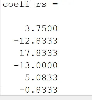
ie a=3.7500, b= -12.8333,c=17.8333, d= =13.000, e=5.0833, g=-0.8333

3. Skewed left-sided difference

The order of accuracy P = Number of nodes in the stencil N - order of derivative Q for one-sided/skewed schemes

So that N=P+Q = 4+2=6

`((partial)^2y)/(partial(x)^2)=a.f(i)+b.f(i-1)+c.f(i-2)+d.f(i-3)+e.f(i-4)+g.f(i-5)`

then we can create Taylor table by expandig each terms by Taylor series

`((partial)^2f)/((partial(x))^2`	f(i)	f'(i).(dx)	f"(i).(dx)^2	f"'(i).(dx)^3	f""(i).(dx)^4	f""'(i).(dx)^5
a.f(i)	a	0	0	0	0	0
b.f(i-1)	b	-b	b/2	-b/6	b/24	-b/120
c.f(i-2)	c	-2c	4c/2	-8c/6	16c/24	-32c/120
d.(f(i-3)	d	-3d	9d/2	-27d/6	81d/24	-243d/120
e.f(i-4)	e	-4e	16e/2	-64e/6	256e/24	-1024e/120
g.f(i-5)	g	-5g	25g/2	-125g/6	625g/24	-3125g/120
Sum of coefficient	0	0	1	0	0	0

Here also 6 unkonwns(a,b,c,d,e,& f0 and 6 equations and that 6 equtions are given below:

a+b+c+d+e+f=0...........................................................................................(1)

0+(-b)+(-2c)+(-3d)+(-4e)+(-5g)=0.................................................................(2)

0+b/2+4c/2+9d/2+16e/2+25g/2=1................................................................(3)

0+(-b/6)+(-8c/6)+(-27d/6)+(-64e/6)+(-125g/6)=0..........................................(4)

0+b/24+16c/24+81d/24+256e/24+625g/24=0.................................................(5)

0+(-b/120)+(-32c/120)+(-243d/120)+(-1024e/120)+(-3125g/120)=0...............(6)

We will solve these equations by using matrix invesrion method

so that A=`[[1,1,1,1,1,1],[0,-1,-2,-3,-4,-5],[0,1/2,4/2,9/2,16/2,25/2],[0,-1/6,-8/6,-27/6,-64/6,-125/6],[0/1/24,16/24,81,24,256/24,625/24],[0,-1/120,-32/120,-243/120,-1024/120,-3125/120]]`

X=`[[a],[b],[c],[d],[e],[g]]`

B=`[[0],[0],[1],[0],[0],[0]]`

We will solve this matrix in MATLAB and we will get the values for the unknowns.

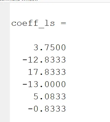
ie a=3.7500, b= -12.8333, c=17.8333,d=-13.000,e=5.0833,g==0.8333

MATLAB Programe:

clear all % clearing workspace
close all % closing all figures and plots
clc       % clearing screen
%% central difference
A_cd=[1 1 1 1 1;-2 -1 0 1 2;4/2 1/2 0 1/2 4/2;-8/6 -1/6 0 1/6 8/6;
    16/24 1/24 0 1/24 16/24];
B_cd=[0;0;1;0;0]; % defining B

%coeff_cd=inv(A_cd)*B_cd;%finding unknown coefficients
coeff_cd=linsolve(A_cd, B_cd);%finding unknown coefficients

%% right skewed
A_rs=[1 1 1 1 1 1;0 1 2 3 4 5;0 1/2 4/2 9/2 16/2 25/2;0 1/6 8/6 27/6 64/6 125/6;
    0 1/24 16/24 81/24 256 /24 625/24;0 1/120 32/120 243/120 1024/120 3125/120];
B_rs=[0;0;1;0;0;0];
coeff_rs=inv(A_rs)*B_rs;
%% left skewed
A_ls=[1 1 1 1 1 1;0 -1 -2 -3 -4 -5;0 1/2 4/2 9/2 16/2 25/2;0 -1/6 -8/6 -27/6 -64/6 -125/6;
    0 1/24 16/24 81/24 256 /24 625/24;0 -1/120 -32/120 -243/120 -1024/120 -3125/120];
B_ls=[0;0;1;0;0;0];
coeff_ls=inv(A_ls)*B_ls;
%% giving a value for x,dx
x=pi/3;
dx=linspace(pi/3,pi/3000,20);
der_analytical=-2*exp(x)*sin(x);%finding analytical derivative
%% defining inline function
f=@(x) exp(x)*cos(x);

%% opening for loop
for i=1:length(dx)
    %% central difference
    deri_cd=coeff_cd(1)*f(x-(2*dx(i)))+coeff_cd(2)*f(x-(1*dx(i)))+coeff_cd(3)*f(x)+coeff_cd(4)*f(x+ (1*dx(i)))+coeff_cd(5)*f(x+(2*dx(i)))
    error_cd(i)=abs(der_analytical-deri_cd);
    %% right skewed
    deri_rs=coeff_rs(1)*f(x)+coeff_rs(2)*f(x+1*dx(i))+coeff_rs(3)*f(x+2*dx(i))+coeff_rs(4)*f(x+3*dx(i))+coeff_rs(5)*f(x+4*dx(i))+coeff_rs(6)*f(x+5*dx(i))
    error_rs(i)=abs(der_analytical-deri_rs);
    %% left skewed
    deri_ls=coeff_ls(1)*f(x)+coeff_ls(2)*f(x-1*dx(i))+coeff_ls(3)*f(x-2*dx(i))+coeff_ls(4)*f(x-3*dx(i))+coeff_ls(5)*f(x-4*dx(i))+coeff_ls(6)*f(x-5*dx(i))
    error_ls(i)=abs(der_analytical-deri_ls);

end % ending for loop
% plotting results
figure(1);
plot(dx,error_cd,'r')
hold on
plot(dx,error_rs,'b')
hold on
plot(dx,error_ls,'m')
hold off
xlabel('dx')
ylabel('error')
legend('cd','rs','ls')

figure(2);
loglog(dx,error_cd,'r')
hold on
loglog(dx,error_rs,'b')
hold on
loglog(dx,error_ls,'m')
hold off
xlabel('dx')
ylabel('error')
legend('cd','rs','ls')

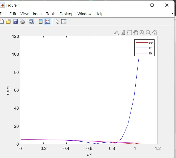
dx vs error plot for different schemes

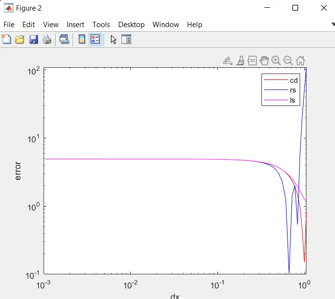
loglog plot for dx vs error for different schemes.

From this plot we can see that when dx value increases the error in right side scheme is increasing.

Why Skewed scheme is useful?

The skewed scheme is useful because it is necessary to compute the grids at the corners also which central differecing scheme is unable to do. Symmetric nodes does not present on the corners so that CD can not be implemented in such conditions.

* Skewed schemes are also uising for problems with boundary conditions.

CONCLUSIONS:

Central difference scheme is better among 3 schemes.

Skewed schemes are better for corners and problems with boundary conditions.

As the value of dx and x changes shape of graphs also changing.

Note: If any error is there in plots please give a proper clarification about error means where is error and why it is coming like information please provide.