Week 3.5 - Deriving 4th order approximation of a 2nd order derivative using Taylor Table method

AIM:

• To create a MATLAB programme for 4th order approximation of a second-order derivative using the following methods:

1. Central difference
2. Skewed right-sided difference
3. Skewed left-sided

OBJECTIVE:

• Using the above-mentioned order of approximations, calculate the second-order derivative of the function f(x) = exp(x)cos x.
• Plot and compare the values and errors of the three derived methods.

THEORY:

• When solving a CFD problem, we may encounter a partial derivative equation with a 2nd order derivative. Because of the complexity of the equation, we may have to use a numerical approach rather than an analytical approach. When dealing with numerical approaches, however, we try to keep the error margin as small as possible.

• As the order of approximation increases, so does the accuracy. As a result, we will derive the three methods of approximation for an analytical function. The procedures are as follows.

1. Central difference: - The nodes chosen here are symmetrical, which means that data is taken from both sides of the point of focus. We obtain using Taylor's method

• Here there are two nodes taken from both sides of the point of focus i.e. f(i).

(NOTE: - To select the number of nodes in consideration, we use the following expression:

• N=p + q -1 for central differencing
• N = p + q for skewed differencing

Here N is no. of nodes, p is the order of derivative and q is the order of approximation.)

Taylor’s table for Central difference:

	f(X)	dx f’(x)	dx2 f’’(x)	dx3 f’’’(x)	dx4 f’’’’(x)	dx5 f’’’’’(x)
af(i-1)	a	-2a	4a/2	-8a/6	16a/24	-32a/120
bf(i-2)	b	-b	b/2	-b/6	b/24	-b/120
cf(i)	c	0	0	0	0	0
df(i-1)	d	d	d/2	d/6	d/24	d/120
ef(i-2)	e	2e	4e/2	8e/6	16e/24	32e/120
af(i-2) +bf(i-1) +cf(i) +df(i+1) + ef(i+2)	0	0	1	0	0	?

• This table transforms into the matrix of type AX=B,

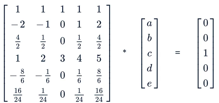
• We get the values of the unknown after further solving.

i.e. Values = a = -0.0833 b= 1.3333 c= -2.5000 d= 1.3333 e= -0.0833

• These coefficients will be further used in code to get the value of the derivative.

2. Skewed right-sided difference: - When the data points of the left nodes are unavailable (due to initial boundary conditions), we must rely on the data set that is available.

Taylor’s table for Skewed right-sided difference:

	f(x)	dx f’ (X)	dx2 f’’ (x)	dx3 f’’’(x)	dx4f’’’’(x)	dx5f’’’’’(x)
af(i)	a	0	0	0	0	0
bf(i+1)	b	b	b/2	b/6	b/24	b/120
cf(i+2)	c	2c	4c/2	8c/6	16c/24	32c/120
df(i+3)	d	3d	9d/2	27d/6	81d/24	243d/120
ef(i+4)	e	4e	16e/2	64e/6	256e/24	1024e/120
ff(i+5)	f	5f	25f/2	125f/6	625f/24	3125f/120
af(i) + bf(i+1) + cf(i+2) + df(i+3) + ef(i+4) +ff(i+5)	0	0	1	0	0	0

• This table transforms into the matrix of type AX=B:

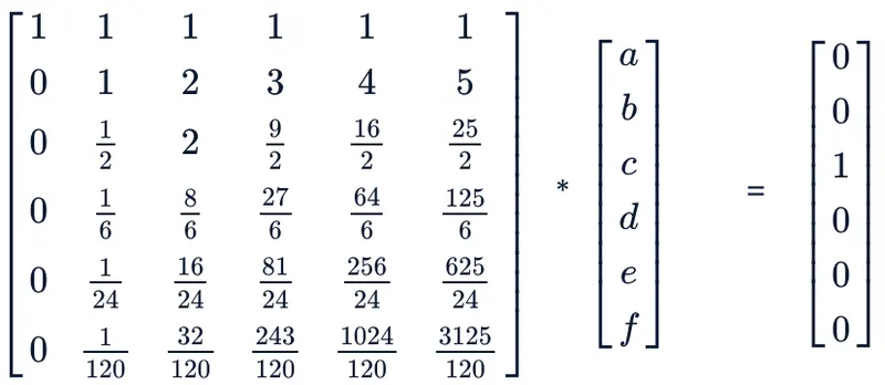
• We obtain the values of the after further solving,

unknown i.e. Values = a = 3.7500 b= -12.8333 c= 17.8333 d= -13.0000 e= 5.0833 f= -0.8333

• These coefficients will be further used in code to get the value of the derivative.

3. Skewed left-sided difference: - When the data point of the correct node is unavailable (due to boundary conditions), we must rely on the available data set.

• Taylor’s table for Skewed right-sided difference:

	f(x)	dx f’ (X)	dx2 f’’ (x)	dx3 f’’’(x)	dx4f’’’’(x)	dx5f’’’’’(x)
af(i-5)	a	-5a	25a/2	-125a/6	625a/24	-3125a/120
bf(i-4)	b	-4b	16b/2	-64b/6	256b/24	-1024b/120
cf(i-3)	c	-3c	9c/2	-27c/6	81c/24	-243c/120
df(i-2)	d	-2d	4d/2	-8d/6	16d/24	-32d/120
ef(i-1)	e	-e	e/2	-e/6	e/24	-e/120
ff(i)	f	0	0	0	0	0
af(i-5) + bf(i-4) + cf(i-3) + df(i-2) + ef(i-1) +ff(i)	0	0	1	0	0	0

• This table transforms into the matrix of type AX=B:

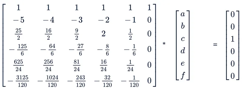
• on further solving we get the values of the,

unknown i.e. Values = a = -0.8333 b= 5.0833 c=13.0000 d= 17.8333 e= -12.8333 f= 3.7500

• These coefficients will be further used in code to get the value of the derivative.

MATLAB CODE:

% inputs

 x=pi/3;

 %stepsize range

 dx=linspace(pi/4,pi/400,2000);

 % Analytical derivative

 %f(x) = exp(x)*cos(x)
 %f'(x)=(exp(x)*cos(x)-(exp(x)*sin(x)=exp(x)*(cosx-sinx)
 %Double derivative f" = -2*exp(x)*sin(x)

 analytical_derivative = -2*exp(x)*sin(x);

 % Skewed right-sided(4th order approimation)
 % Solving for the coefficients

 A=[1 1 1 1 1 1;0 1 2 3 4 5; 0 1/2 4/2 9/2 16/2 25/2; 0 1/6 8/6 27/6 64/6 125/6; 0 1/24 16/24 81/24 256/24 625/24; 0 1/120 32/120 243/120 1024/120 3125/120];
 B=[0;0;1;0;0;0];
 x_r=inv(A)*B;

 % Skewed left-sided(4th order approimation)
 % Solving for the coefficients

 C=[1 1 1 1 1 1;0 -1 -2 -3 -4 -5; 0 1/2 4/2 9/2 16/2 25/2; 0 -1/6 -8/6 -27/6 -64/6 -125/6; 0 1/24 16/24 81/24 256/24 625/24; 0 -1/120 -32/120 -243/120 -1024/120 -3125/120];
 D=[0;0;1;0;0;0];
 x_l=inv(C)*D;

 % central differencing(4th order approimation)
 % Solving for the coefficients

 E=[1, 1, 1, 1, 1; -2, -1, 0, 1, 2; 4/2, 1/2, 0, 1/2, 4/2; -8/6, -1/6, 0, 1/6, 8/6; 16/24, 1/24, 0, 1/24, 16/24];
 F=[0;0;1;0;0];
 x_c=E^-1*F;

 % Anonymous Function

 f=@(x) exp(x).*cos(x);


 % numerical derivative

 right_difference=(x_r(1)*f(x)+x_r(2)*f(x+dx)+x_r(3)*f(x+2.*dx)+x_r(4)*f(x+3.*dx)+x_r(5)*f(x+4.*dx)+x_r(6)*f(x+5.*dx))./(dx.^2)

 left_difference=(x_r(1)*f(x)+x_r(2)*f(x-dx)+x_r(3)*f(x-2.*dx)+x_r(4)*f(x-3.*dx)+x_r(5)*f(x-4.*dx)+x_r(6)*f(x-5.*dx))./(dx.^2)

 cent_difference=(x_c(1)*f(x-2.*dx)+x_c(2)*f(x-1.*dx)+x_c(3)*f(x)+x_c(4)*f(x+dx)+x_c(5)*f(x+2.*dx))./(dx.^2)



 % absolute error

 error_r=abs(analytical_derivative-right_difference);
 error_l=abs(analytical_derivative-left_difference);
 error_c=abs(analytical_derivative-cent_difference);
 error=[error_r;error_l;error_c];



 figure(1)
 loglog(dx,error_r)
 hold on
 loglog(dx,error_l)
 loglog(dx,error_c)
 ylabel('Absolute Error (Log Scale)')
 xlabel('Grid Spacing (dx in Log Scale)')
 legend('Right Differencing','Left Differencing','Central Differencing')

RESULT:

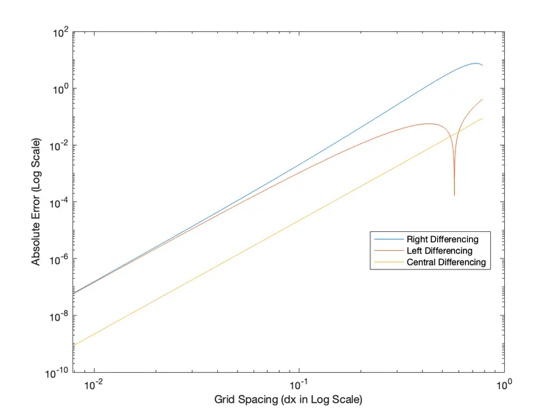
CONCLUSION:

• As shown in the figure above, the error for the central difference method is much lower than for the skewed methods.
• Skewed right and left difference methods produce nearly identical results in terms of error for a small time step value.
• When data from grid points is only available from either the left or right end, i.e. at nodes closer to the boundaries, we use skewed schemes for computations that require high-order approximations. Having a symmetric stencil for computation, as we do for central differencing schemes or having a low order accuracy, is not possible in these scenarios. For better scheme consistency, the values of dx are kept as low as possible to provide proper computational plots.
• A skewed scheme is useful when we have only one direction to go and must predict using the boundary condition. As a result, the skewed scheme will be useful, and the central differencing scheme will be ineffective for such an application because it requires information from both directions of the point.