Week 3.5 - Deriving 4th order approximation of a 2nd order derivative using Taylor Table method
Fourth order approximation of second order derivative
Aim:
To derive fourth-order accurate scheme of second-order derivative using Finite Difference Method (FDM) and program the same in MATLAB. Three different stencils–Central-difference, skewed-left and skewed-right differencing scheme–were used in this project and the absolute error between the scheme and the exact solution was calculated and compared for the three different schemes.
Theory:
Finite differences are a class of numerical techniques for solving differential equations by approximating the derivatives into finite differences. This method, with the help of Taylor series, converts the differential equation into a system of linear equations that can be solved in computers. The two sources of error in a FDM are truncation error and round-off error. The truncation errors occurs due to the selection of finite number of terms in the Taylor series to approximate the derivative. Round-off error is caused due to computer rounding of decimal quantities [1]. Using Taylor series, a first-order derivative can be written as
`f’(x) = (f(x+h) – f(x))/(h) + O(h)`
One must discretize the domain into discrete points to approximate the solution of a problem by FDM. It can be observed from the above equation that the truncation error is proportional to the step size (`h`). The truncation error can be reduced by decreasing the step-size or by including higher number of neighbouring points in the approximation. A formula corelating the desired accuracy, order of derivative and the number of points to be chosen is given by
Symmetric stencil:
Order of accuracy (`p`) = Number of points (`N`) – order of derivative (`Q`) + 1
Unsymmetric stencil:
Order of accuracy (`p`) = Number of points (`N`) – order of derivative (`Q`)
Note: Symmetric stencil has equal number of terms on either side of the point of interest. Unsymmetric stencil has more number of terms on one side of the point of interest.
Procedure:
In this project, a 4th order accurate scheme is desired for approximating the second order differential equation. Using the above formula, number of terms in the stencil can be determined.
Central Scheme (symmetric):
Number of points (`N`) = 4 + 2 -1 = 5
The second order derivative can be then written as
`f’’(x) = (a*f(x-2*Delta x) + b*f(x-Delta x) + c*f(x) + d*f(x+Delta x) + e*f(x+2* Delta x) + O(Delta x^4))/(Delta x^2)`
Each of the terms on the right-hand side are expanded using taylor series [2] and compared with the terms on the left-hand side to determine the co-efficient. The taylor table method can be adopted
for this purpose [3]. In order to make the process easier for computation, the following equation was used in the taylor table method
`Delta x^2 * f’’(x) = a*f(x-2*Delta x) + b*f(x-Delta x) + c*f(x) + d*f(x+Delta x) + e*f(x+2* Delta x)`
The following table illustrates the taylor table method for the central scheme
|
`f(x)` |
`Delta x*f‘(x)` |
`Delta x^2*f‘‘(x)` |
`Delta x^3*f‘‘‘(x)` |
`Delta x^4*f‘‘‘‘(x)` |
`Delta x^5*f‘‘‘‘‘(x)` |
|
|
`a * f(x)` |
`a` |
0 |
0 |
0 |
0 |
0 |
|
`b* f(x+ Delta x)` |
`b` |
`b` |
`b/2` |
`b/6` |
`b/24` |
`b/120` |
|
`c* f(x+2* Delta x)` |
`c` |
`2*c` |
`4*c/2` |
`8*c/6` |
`16*c/24` |
`32*c/120` |
|
`d* f(x- Delta x)` |
`d` |
`-d` |
`d/2` |
`-d/6` |
`d/24` |
`-d/120` |
|
`e* f(x-2*Delta x)` |
`e` |
`-2*e` |
`4*e/2` |
`-8*e/6` |
`16*e/24` |
`-32*e/120` |
|
LHS |
0 |
0 |
1 |
0 |
0 |
- |
Each column was written as individual equations as shown. As there are only five unknowns, five equations would suffice.
`a+b+c+d+e = 0`
`b + 2*c - d – 2*e = 0`
`b/2 + 4*c/2 + d/2 + 4*e/2=0`
`b/6 + 8*c/6 - d/6 - 8*e/6 = 0`
`b/24 + 16*c/24 + d/24 + 16*e/24 = 0`
The above five equations with 5 unkowns were solved in MATLAB and the coefficients were determined.
A similar procedure was adopted for the unsymmetric schemes also.
Forward scheme (unsymmetric):
Number of points (`N`) = 4 + 2 = 6
`Delta x^2 * f’’(x) = a*f(x) + b*f(x+Delta x) + c*f(x+2*Delta x) + d*f(x+3*Delta x) + e*f(x+4* Delta x) + g*f(x + 5*Delta x)`
The following table illustrates the taylor table method for the central scheme
|
`f(x)` |
`Delta x*f‘(x)` |
`Delta x^2*f‘‘(x)` |
`Delta x^3*f‘‘‘(x)` |
`Delta x^4*f‘‘‘‘(x)` |
`Delta x^5*f‘‘‘‘‘(x)` |
|
|
`a * f(x)` |
`a` |
0 |
0 |
0 |
0 |
0 |
|
`b* f(x+ Delta x)` |
`b` |
`b` |
`b/2` |
`b/6` |
`b/24` |
`b/120` |
|
`c* f(x+2* Delta x)` |
`c` |
`2*c` |
`4*c/2` |
`8*c/6` |
`16*c/24` |
`32*c/120` |
|
`d* f(x+3* Delta x)` |
`d` |
`3*d` |
`9*d/2` |
`27*d/6` |
`81*d/24` |
`243*d/120` |
|
`e* f(x+4*Delta x)` |
`e` |
`4*e` |
`16*e/2` |
`64*e/6` |
`256*e/24` |
`1024*e/120` |
|
`g* f(x+5*Delta x)` |
`g` |
`5*g` |
`25*g/2` |
`125*g/2` |
`625*g/2` |
`3125*g/2` |
|
LHS |
0 |
0 |
1 |
0 |
0 |
0 |
Each column was written as individual equations as shown. As there are only five unknowns, five equations would suffice.
`a+b+c+d+e = 0`
`b + 2*c +3* d + 4*e +5*g = 0`
`b/2 + 4*c/2 + 9*d/2 + 16*e/2 + 25*g/2 =0`
`b/6 + 8*c/6 + 27*d/6 + 64*e/6 + 125*g/6 = 0`
`b/24 + 16*c/24 + 81*d/24 + 64*e/24 + 625*g/2= 0`
`b/120 + 32*c/120 + 243*d/120 + 1024*e/120 + 3125*g/2 = 0`
Backward scheme (unsymmetric):
Number of points (`N`) = 4 + 2 = 6
`Delta x^2 * f’’(x) = a*f(x) + b*f(x-Delta x) + c*f(x-2*Delta x) + d*f(x-3*Delta x) + e*f(x-4* Delta x) + g*f(x - 5*Delta x)`
The following table illustrates the taylor table method for the central scheme
|
`f(x)` |
`Delta x*f‘(x)` |
`Delta x^2*f‘‘(x)` |
`Delta x^3*f‘‘‘(x)` |
`Delta x^4*f‘‘‘‘(x)` |
`Delta x^5*f‘‘‘‘‘(x)` |
|
|
`a * f(x)` |
`a` |
0 |
0 |
0 |
0 |
0 |
|
`b* f(x- Delta x)` |
`b` |
`-b` |
`b/2` |
`-b/6` |
`b/24` |
`-b/120` |
|
`c* f(x-2* Delta x)` |
`c` |
`-2*c` |
`4*c/2` |
`-8*c/6` |
`16*c/24` |
`-32*c/120` |
|
`d* f(x-3* Delta x)` |
`d` |
`-3*d` |
`9*d/2` |
`-27*d/6` |
`81*d/24` |
`-243*d/120` |
|
`e* f(x-4*Delta x)` |
`e` |
`-4*e` |
`16*e/2` |
`-64*e/6` |
`256*e/24` |
`-1024*e/120` |
|
`g* f(x-5*Delta x)` |
`g` |
`-5*g` |
`25*g/2` |
`-125*g/2` |
`625*g/2` |
`-3125*g/2` |
|
LHS |
0 |
0 |
1 |
0 |
0 |
0 |
0
Each column was written as individual equations as shown. As there are only five unknowns, five equations would suffice.
`a+b+c+d+e = 0`
`-b - 2*c -3* d - 4*e -5*g = 0`
`b/2 + 4*c/2 + 9*d/2 + 16*e/2 + 25*g/2 =0`
`-b/6 - 8*c/6 - 27*d/6 - 64*e/6 - 125*g/6 = 0`
`b/24 + 16*c/24 + 81*d/24 + 64*e/24 + 625*g/2= 0`
`-b/120 - 32*c/120 - 243*d/120 - 1024*e/120 - 3125*g/2 = 0`
MATLAB Implemetation:
The system of equations derived from each scheme were solved using MATLAB. For this purpose, matrices were created for the coefficients on the left-hand side and a vector for the values on the right-hand side. The following code-snippet shows the procedure adopted to determine the coefficients
%% central scheme
 A_center = [1 1 1 1 1;...
             0 -1 -2 1 2;...
             0 1/2 4/2 1/2 4/2;...
             0 -1/6 -8/6 1/6 8/6;...
             0 1/24 16/24 1/24 16/24];

 b_center = [0;0;1;0;0];

 coeff_center = A_center\b_center;
%[num_center,dem_center] = rat(coeff_center);

%% shewed right stencil - forward
A_skew_right = [1 1 1 1 1 1;...
                0 1 2 3 4 5;...
                0 1/2 4/2 9/2 16/2 25/2;...
                0 1/6 8/6 27/6 64/6 125/6;...
                0 1/24 16/24 81/24 256/24 625/24;...
                0 1/120 32/120 243/120 1024/120 3125/120];

b_skew_right = [0;0;1;0;0;0];
coeff_skew_right = A_skew_right\b_skew_right;
%[num_right,dem_right] = rat(coeff_skew_right);

%% shewed left scheme - backward
 A_skew_left = [1 1 1 1 1 1;...
                0 1 2 3 4 5;...
                0 1/2 4/2 9/2 16/2 25/2;...
                0 1/6 8/6 27/6 64/6 125/6;...
                0 1/24 16/24 81/24 256/24 625/24;...
                0 1/120 32/120 243/120 1024/120 3125/120];

b_skew_left = [0;0;1;0;0;0];
coeff_skew_left = A_skew_left\b_skew_left;
%[num_left,dem_left] = rat(coeff_skew_left);
A matrix and b vector were initialised using the values from the system of equations derived in the previous section. The “\” operator was used to solve the matrix equation `x = b"\"A` and the unknown coefficients were calculated [4]. Since MATLAB outputs decimal values, the function “rat” was used to convert into fractions. These fractions were used only for better representation of the results and were not used in further calculation.
Three different functions were programmed for the three schemes and the determined coefficients were directly passed to it. The function then outputs the value of the second-order derivative calculated using the corresponding scheme. This was done to avoid any round-off error caused by manual input. The three functions are shown in the following code snippet
%% functions

    function central_diff = fourth_order_central_difference(x,dx,A_center)
        central_diff = (A_center(1)*userfunc(x) + A_center(2)*userfunc(x-dx) +
                         A_center(3)*userfunc(x-2*dx) + A_center(4)*userfunc(x+dx) +
                          A_center(5)*userfunc(x+2*dx))/(dx^2);

    end

    function forward_diff = fourth_order_forward_difference(x,dx,A_skew_right)
        forward_diff = (A_skew_right(1)*userfunc(x) + A_skew_right(2)*userfunc(x+dx) +
                        A_skew_right(3)*userfunc(x+2*dx) +
                        A_skew_right(4)*userfunc(x+3*dx) +
                        A_skew_right(5)*userfunc(x+4*dx) +
                        A_skew_right(6)*userfunc(x+5*dx))/(dx^2);
    end

    function backward_diff = fourth_order_backward_difference(x,dx,A_skew_left)
        backward_diff = (A_skew_left(1)*userfunc(x) + A_skew_left(2)*userfunc(x-dx) +
                         A_skew_left(3)*userfunc(x-2*dx) +
                         A_skew_left(4)*userfunc(x-3*dx) +
                         A_skew_left(5)*userfunc(x-4*dx) +
                         A_skew_left(6)*userfunc(x-5*dx))/(dx^2);
    end
These functions call the user-function “userfunc” which calculates the value of the user-function at the given points. The user-function used in this project was `exp(x)*cos(x)` and it was implemented in MATLAB as
function func_value = userfunc(x)
    func_value = exp(x)*cos(x);
end
In order to compute the absolute error, the second derivative of the user-function was calculated and implemented as
%% analytical solution
analytical_soln = -2*exp(x)*sin(x);
The analytical solution and the approximations were calculated at `x=pi/3`. In order to compare the behavior of the schemes at different step-size, `Delta x` was varied from `pi/400 to pi/40`
A main script was created which calls the other functions and determines the absolute error value for the different schemes.
%% main function
central_difference = zeros(1,length(dx));
forward_difference = zeros(1,length(dx));
backward_difference = zeros(1,length(dx));

% Approximate value calculation
for i = 1:length(dx)
    central_difference(i) = fourth_order_central_difference(x,dx(i),coeff_center);

    forward_difference(i) = fourth_order_forward_difference(x,dx(i),coeff_skew_right);

    backward_difference(i) = fourth_order_backward_difference(x,dx(i),coeff_skew_left);

end

%% absolute error
error_central_difference = abs(analytical_soln - central_difference);
error_forward_difference = abs(analytical_soln - forward_difference);
error_backward_difference = abs(analytical_soln - backward_difference);
First, three matrices were initialised as zeros of length corresponding the stepsize vector. This is done to increase the execution speed of the program. Next for loop is called which calls the three functions and calculates the approximate values of the derivative and stores them in the respective array. Then the absolute error was calculated for each scheme.
Results:
The coefficients determined from MATLAB are shown in the following equations
Central differencing scheme
`f’’(x) = (-1*f(x-2*Delta x) + 16*f(x-Delta x) + -30*f(x) + 16*f(x+Delta x) -1*f(x+2* Delta x))/(12*Delta x^2)`
Forward differencing scheme
` f’’(x) = (45*f(x) -154*f(x+Delta x) + 214*f(x+2*Delta x) -156 *f(x+3*Delta x) + 61*f(x+4* Delta x) - 10*f(x + 5*Delta x))/( 12*Delta x^2)`
Backward differencing scheme
` f’’(x) = (45*f(x) -154*f(x-Delta x) + 214*f(x-2*Delta x) -156*f(x-3*Delta x) + 61*f(x-4* Delta x) -10 g*f(x - 5*Delta x))/(12*Delta x^2 )`
Then the absolute error calculated was plotted as a function of stepsize using the loglog plot in MATLAB. The following code-snippet shows this implementation
%% plot errors
figure
loglog(dx,error_central_difference,'-r')
hold on;
loglog(dx,error_forward_difference,'-b')
hold on;
loglog(dx,error_backward_difference,'-k')
xlabel('log(dx)')
ylabel('log(absolute error)')
legend('central-differencing','forward-differencing','backward-differencing','Location','best')
The plots obtained from this program is shown below
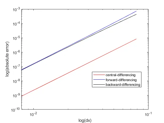
It can be observed that the central differencing scheme produces the least error compared to the other two schemes. The rate of decrease in error is the same in all the schemes.
Although the error in a central differencing scheme is less, it can not be employed at the boundaries because of the lack of points outside the boundary [5]. The selection of scheme depends on the type of problem and also on the location inside the domain.
References: