Week 3.5 - Deriving 4th order approximation of a 2nd order derivative using Taylor Table method

• Agenda:
• Need for higher order Schmes because Accuracy that Plays an important role
• Accuracy obtained by:
• Requires fewer grid points in total
• Captures the information with resolution,Ie.,Information is nothing but flows in our domain is described by method of characterstics.
• When computing derivative at point (i) & collects information by FDs,BDs,& CDs
• Skewed & Symmetrical

Skewed:

1. A Skewed Schmes is one which takes unequal no of grid points on either side
2. They are Forward differnce schmes
3. Backward differnce schmes
4. Central differnce schmes.

Concept of Numerical Stencil:

• Numerical stencils are Pictorial representation of finite Differnce points
• Its shows the information transfer b/w grids for the type of discretization schmes used.
• The no of points (N)required to obtain an accuracy (A) for the order of Derivate (O) is given by Thumb Rule.

N=O+A(Skewed)

N=O+A-1(Symmetrical)

N= number of points.

A=Order of Acccuracy.

O=oder of derivative.

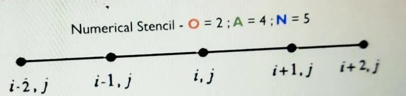
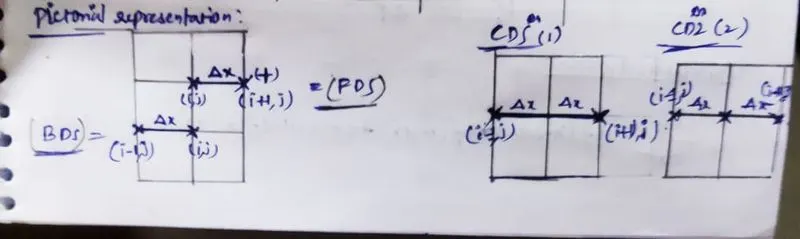
Here computing 4th order Accurate/Approximation of Second order derivative for five points.

Here higher order accurate formulations can be derived by using Taylors table.

clc
close all
clear all

% CDS
A=[1 1 1 1 1;-2 -1 0 1 2;4/2 1/2 0 1/2 4/2;-8/6 -1/6 0 1/6 8/6;16/24 1/24 0 1/24 16/24];
B=[0;0;1;0;0];
X=inv(A)*B

% SL
C=[1 1 1 1 1 1;0 -1 -2 -3 -4 -5;0 1/2 4/2 9/2 16/2 25/2;0 -1/6 -8/6 -27/6 -64/6 -125/6;0 1/24 16/24 81/24 256/24 625/24;0 -1/120 -32/120 -243/120 -1024/120 -3125/120];
D=[0;0;1;0;0;0];
Y=inv(C)*D

% SR
E=[1 1 1 1 1 1;0 1 2 3 4 5;0 1/2 4/2 9/2 16/2 25/2;0 1/6 8/6 27/6 64/6 125/6;0 1/24 16/24 81/24 256/24 625/24;0 1/120 32/120 243/120 1024/120 3125/120];
F=[0;0;1;0;0;0];
Z=inv(E)*F

x = pi/3;%initial point 
dx = linspace(pi/3,pi/4000,100) ;%  difference in points(dx)

f = @(x) exp(x).*cos(x);% function of derivative.


%ananlytical_2nd_derivative:
analytical_derivative=-2*exp(x)*sin(x);


%Numerical:
central_differncing = (X(1)*f(x-2*dx) +X(2)*f(x-dx)+ X(3)*f(x) +X(4)*f(x+dx) +X(5)*f(x+2*dx))./(dx.^2);
error_CDS = abs(central_differncing-analytical_derivative);

% Numerical derivative:
backward_differencing = (Y(1)*f(x) + Y(2)*f(x-dx) + Y(3)*f(x-2*dx) + Y(4)*f(x-3*dx) + Y(5)*f(x-4*dx) + Y(6)*f(x-5*dx))./(dx.^2);
error_SL = abs(backward_differencing - analytical_derivative);

% Numerical derivative:
forward_differencing = (Z(1)*f(x) + Z(2)*f(x+dx) + Z(3)*f(x+2*dx) + Z(4)*f(x+3*dx) + Z(5)*f(x+4*dx) + Z(6)*f(x+5*dx))./(dx.^2);
error_SR= abs(forward_differencing-analytical_derivative);


figure(1)
loglog(dx,error_CDS,dx,error_SR,dx,error_SL)
hold on
grid on
xlabel('dx')
ylabel('error')
legend('CDSs','Skewed Right','Skewed Left')
title('Comparison of 4th order accurate schemes')

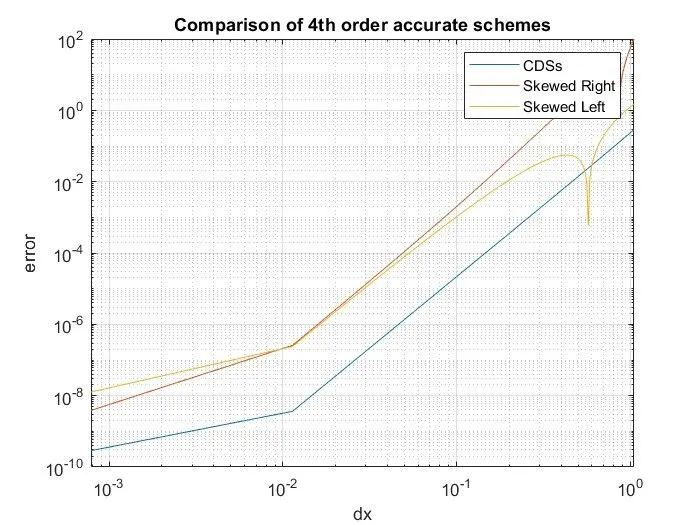
Explanation of code:

• The above code explains that dx (pi/40,pi/50,pi/60 ....so on upto pi/4000) it varies ie., vary between two nodes & calculate (pi/40 ) for each given points of the given differntial equations shouls be computed , similarly for pi/50,pi/60,pi/70...so on.As the (dx) ie., distance decreases the no of nodes increases in the field domain & the Error gets decreases ie.,closer,continious & more Accurate results we produced.
• Its calculates for the 5 points.
• Approximation method.
• As the higher order Schmes gives an an accurate results and ans also increases in the no of nodes.