Week 3.5 - Deriving 4th order approximation of a 2nd order derivative using Taylor Table method
Deriving 4th order approximation of a 2nd order derivative using Taylor Table method :
GIVEN PROBLEM:
Derive the following 4th order approximations of the second-order derivative.
1. Central difference
2. Skewed right-sided difference
3. Skewed left-sided difference
After deriving these schemes, prove that your skewed schemes are fourth-order accurate i.e the thumb rule given in HINT (ii).
Once you have done this, write a program in Matlab to evaluate the second-order derivative of the analytical function exp(x)*cos(x) and compare it with the 3 numerical approximations that you have derived.
Provide a plot that compares the absolute error between the above-mentioned schemes
In your own words, describe why a skewed scheme is useful? What can a skewed scheme do that a CD scheme cannot?
1. CENTRAL DIFFERENCE:
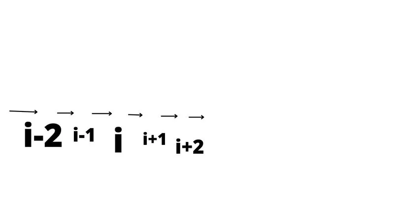
As we are computing fourth order approximation of second order derivative by central difference method at point (i) so
we are taking five points where two are left of (i) and two are right of (i) . Based on the above stencil our hypothesis equation
will be : ( ∂ˆ2 u/ ∂xˆ2 )=a*f(i-2)+b*f(i-1)+c*f(i)+d*f(i+1)+e*f(i+2) ..............(1)
In order to find the coefficients (a,b,c,d,e) we have to use Taylor table method.Taylor series expansion of each term of equation (1) is :
a*f(i-2 )= a*f(i)-a*( 2Δx/1!)*f '(i)+a*f ''(i)*(2Δx)^2/2! -a*f '''(i)*(2Δx)^3/3!+a*f''''*(2Δx)^4/4!-a*f '''''(i)*(2Δx)^5/5!
+a*f ''''''(i)*(2Δx)^6/6!+ .........
b*f(i-1)= b*f(i)-b*( Δx/1!)*f '(i)+b*f ''(i)*(Δx)^2/2! -b*f '''(i)*(Δx)^3/3!+b*f''''*(Δx)^4/4!-b*f '''''(i)*(Δx)^5/5!
+b*f ''''''(i)*(Δx)^6/6!+ .........
c*f(i)=c*f(i)
d*f(i+1)= d*f(i)+d*( Δx/1!)*f '(i)+d*f ''(i)*(Δx)^2/2! +d*f '''(i)*(Δx)^3/3!+d*f''''*(Δx)^4/4!+d*f '''''(i)*(Δx)^5/5!
+d*f ''''''(i)*(Δx)^6/6!+ .........
e*f(i+2)=e*f(i)+e*( 2Δx/1!)*f '(i)+e*f ''(i)*(2Δx)^2/2! +e*f '''(i)*(2Δx)^3/3!+e*f''''*(2Δx)^4/4!+e*f '''''(i)*(2Δx)^5/5!
+e*f ''''''(i)*(2Δx)^6/6!+ .........
By arranging above expansions on Taylor table we get:
| f(i) | Δxf(i) | Δx^2 f''(i) | Δx^3 f '''(i) | Δx^4 f ''''(i) | Δx^5 f '''''(i) | Δx^6 f''''''(i) | |
| a* f(i-2) | a | -2a | 2a | -(8a/6) | 16a/24 | -32a/120 | 64a/240 |
| b*f(i-1) | b | -b | b/2 | -b/6 | b/24 | -b/120 | b/240 |
| c*f(i) | c | 0 | 0 | 0 | 0 | 0 | 0 |
| d*f(i+1) | d | d | d/2 | d/6 | d/24 | d/120 | d/240 |
| e*f(i+2) | e | 2e | 2e | 8e/6 | 16e/24 | -32e/120 | 64e/240 |
|
∑a* f(i-2)+b*f(i-1)+c*f(i)+d*f(i+1) +e*f(i+2) =(∂ˆ2 u/ ∂xˆ2 ) |
0 | 0 | 1 | 0 | 0 | ? | ? |
Here we assume 5 terms as our hypothesis so we dont know the last two term.BY summing the unknowns column wise we are getting the following equations :
a+b+c+d+e=0.........(i)
-2a-b+0+d+2e=0......(ii)
2a+b/2+0+d/2+2e=1.......(iii)
-(8a/6)-b/6+0+d/6+8e/6......(iv)
16a/24+b/24+0+d/24+16e/24=0.......(v)
To solve the above equations we have to solve the equations in matrix form AX=B
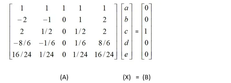
After solving the matrix we get the coefficients as
a=-0.083333
b=1.333333
c=-2.500000
d=1.333333
e=-.083333
Now dividing the hypothysis (1) by( Δx)^2 we get:
( ∂ˆ2 u/ ∂xˆ2 )=(a*f(i-2)+b*f(i-1)+c*f(i)+d*f(i+1)+e*f(i+2))/( Δx)^2
or, ( ∂ˆ2 u/ ∂xˆ2 )=(-.083333*f(i-2)+1.333333*f(i-1)-2.500000*f(i)+1.333333*f(i+1)-.083333*f(i+2))/( Δx)^2
From here we can see that a=e & b=d
finding order of approximation:
Now again from the taylor equation we get
( ∂ˆ2 u/ ∂xˆ2 )=(a+b+c+d+e) *f(i)+(-2a+b+0+d+2e)f '(i) *(Δx)+(2a+b/2+0+d/2+2e)*f ''(i)*(Δx)^2+(-(8a/6)-b/6+0+d/6+8e/6)*f '''(i)*(Δx)^3+(16a/24+b/24+0+d/24+16e/24)f ''''(i)*(Δx)^4+(-32a/120-b/120+0+d/120+32e/120)*f '''''(i)*Δx)^5+(64a/120+b/240+0+d/240+64e/240)*f ''''''(i)*Δx)^6
on substituting the values of (i),(ii),(iii),(iv),(v) on the above equation we get:
( ∂ˆ2 u/ ∂xˆ2 )=(2a+b/2+0+d/2+2e)*f ''(i)*(Δx)^2+(-32a/120-b/120+0+d/120+32e/120)*f '''''(i)*Δx)^5+(64a/120+b/240+0+d/240+64e/240)*f ''''''(i)*Δx)^6
Dividing it by (Δx)^2 we get:
( ∂ˆ2 u/ ∂xˆ2 )=(2a+b/2+0+d/2+2e)*f ''(i)*(Δx)^2+(64a/120+b/240+0+d/240+64e/240)*f ''''''(i)*(Δx)^4
In the above equation the value of (Δx)^4 is truncation error . As the order of truncation error is four so the equation is
fourth order approximation.
2.skewed right sided difference:
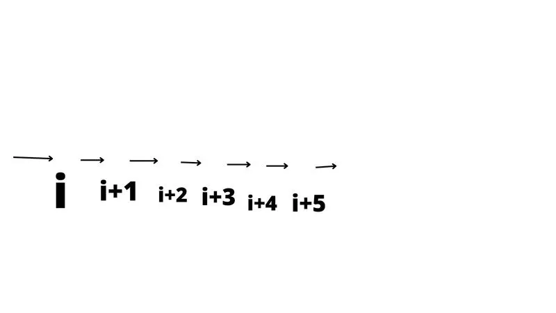
According to above stensil our hypothetical equation is :
( ∂ˆ2 u/ ∂xˆ2 )=a*f(i)+b*f(i+1)+c*f(i+2)+d*f(i+3)+e*f(i+4)+g*f(i+ 5)..............(1)
In order to find the coefficients (a,b,c,d,e,g) we have to use Taylor table method.Taylor series expansion of each term of equation (1) is :
a*f(i)=a*f(i)......
b*f(i+1)= b*f(i)+b*( Δx/1!)*f '(i)+b*f ''(i)*(Δx)^2/2! +b*f '''(i)*(Δx)^3/3!+b*f''''*(Δx)^4/4!+b*f '''''(i)*(Δx)^5/5!
+b*f ''''''(i)*(Δx)^6/6!+ .........
c*f(i+2)=c*f(i)+c*( 2Δx/1!)*f '(i)+c*f ''(i)*(2Δx)^2/2! +c*f '''(i)*(2Δx)^3/3!+c*f''''*(2Δx)^4/4!+c*f '''''(i)*(2Δx)^5/5!
+c*f ''''''(i)*(2Δx)^6/6!+ .........
d*f(i+3)=d*f(i)+d*( 3Δx/1!)*f '(i)+d*f ''(i)*(3Δx)^2/2! +d*f '''(i)*(3Δx)^3/3!+d*f''''*(3Δx)^4/4!+d*f '''''(i)*(3Δx)^5/5!
+d*f ''''''(i)*(3Δx)^6/6!+ .........
e*f(i+4)=e*f(i)+e*( 4Δx/1!)*f '(i)+e*f ''(i)*(4Δx)^2/2! +e*f '''(i)*(4Δx)^3/3!+e*f''''*(4Δx)^4/4!+e*f '''''(i)*(4Δx)^5/5!
+e*f ''''''(i)*(4Δx)^6/6!+ .........
g*f(i+5)=g*f(i)+g*( 5Δx/1!)*f '(i)+g*f ''(i)*(5Δx)^2/2! +g*f '''(i)*(5Δx)^3/3!+g*f''''*(5Δx)^4/4!+g*f '''''(i)*(5Δx)^5/5!
+g*f ''''''(i)*(5Δx)^6/6!+ .........
By arranging above expansions on Taylor table we get:
| f(i) | Δxf(i) | Δx^2 f ''(i) | Δx^3 f'''(i) | Δx^4 f''''(i) | Δx^5 f'''''(i) | Δx^6 f''''''(i) | |
| ( a )f(i) | a | 0 | 0 | 0 | 0 | 0 | 0 |
| (b) f(i+1) | b | b | b/2 | b/6 | b/24 | b/120 | b/720 |
| (c) f(i+2) | c | 2c | 4c/2 | 8c/6 | 16c/24 | 32c/120 | 64c/720 |
|
(d) f(i+3) |
d | 3d | 9d/2 | 27d/6 | 81d/24 | 243d/120 | 729d/720 |
| (e) f(i+4) | e | 4e | 16e/2 | 64e/6 | 256e/24 | 1024e/120 | 4096e/720 |
| (g) f(i+5) | g | 5g | 25g/2 | 125g/6 | 625g/24 | 3125g/120 | 15625g/720 |
| ∑( a )f(i)+ (b) f(i+1)+(c) f(i+2)+(d) f(i+3)+(e) f(i+4)+(g) f(i+5) | 0 | 0 | 1 | 0 | 0 | 0 | ? |
Here we assume 6 terms as our hypothesis so we dont know the last term.BY summing the unknowns column wise we are getting the following equations :
a+b+c+d+e+g=0.........(i)
0+b+2c+3d+4e+5g=0.......(ii)
0+b/2+2c+9d/2+8c+25g/2=1......(iii)
0+b/6+8c/6+27d/6+64e/6+125g/6=0.....(iv)
0+b/24+16c/24+81d/24+256e/24+625g/24=0......(v)
0+b/120+32c/120+243d/120+1024e/120+3125g/120=0.......(vi)
To solve the above equations we have to solve the equations in matrix form AX=B
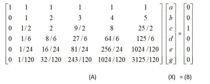
After solving the matrix we get the coefficients as
a=3.75000
b=-12.83333
c=17.83333
d=-13.00000
e=5.08333
g=-0.83333
Now dividing the hypothysis (1) by( Δx)^2 we get:
( ∂ˆ2 u/ ∂xˆ2 )=(a*f(i)+b*f(i+1)+c*f(i+2)+d*f(i+3)+e*f(i+4)+g*f(i+5)/( Δx)^2
or, ( ∂ˆ2 u/ ∂xˆ2 )=(3.75000*f(i)-12.83333*f(i+1)+17.83333*f(i+2)-13.00000*f(i+3)-5.08333*f(i+4)-0.83333*f(i+5))/( Δx)^2
finding order of approximation:
Now again from the taylor equation we get
( ∂ˆ2 u/ ∂xˆ2 )=(a+b+c+d+e+g) *f(i)+(0+b+2c+3d+4e+5g)f '(i) *(Δx)+(0+b/2+4c/2+9d/2+16e/2+25g/2)*f ''(i)*(Δx)^2+(0+b/6+8c/6+27d/6+64e/6+125g/6)*f '''(i)*(Δx)^3+(0+b/24+16c/24+81d/24+256e/24+625g/24)f ''''(i)*(Δx)^4+(b/120+32c/120+243d/120+1024e/120+3125g/120)*f '''''(i)*Δx)^5+(b/720+64c/720+729d/720+4096e/720+15625g/720)*f ''''''(i)*Δx)^6
on substituting the values of (i),(ii),(iii),(iv),(v) on the above equation we get:
( ∂ˆ2 u/ ∂xˆ2 )=(0+b/2+4c/2+9d/2+16e/2+25g/2)*f ''(i)*(Δx)^2+ (b/720+64c/720+729d/720+4096e/720+15625g/720)*f ''''''(i)*Δx)^6
Dividing it by (Δx)^2 we get:
( ∂ˆ2 u/ ∂xˆ2 )=(0+b/2+4c/2+9d/2+16e/2+25g/2)*f ''(i)+ (b/720+64c/720+729d/720+4096e/720+15625g/720)*f ''''''(i)*Δx)^4
In the above equation the value of (Δx)^4 is truncation error . As the order of truncation error is four so the equation is
fourth order approximation.
3.skewed left sided difference:
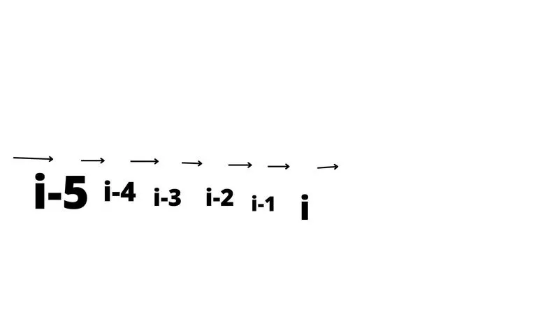
According to above stensil our hypothetical equation is :
( ∂ˆ2 u/ ∂xˆ2 )=a*f(i-5)+b*f(i-4)+c*f(i-3)+d*f(i-2)+e*f(i-1)+g*f(i)..............(1)
In order to find the coefficients (a,b,c,d,e,g) we have to use Taylor table method.Taylor series expansion of each term of equation (1) is :
a*f(i-5)=a*f(i)-a*( 5Δx/1!)*f '(i)+a*f ''(i)*(5Δx)^2/2! -a*f '''(i)*(5Δx)^3/3!+a*f''''*(5Δx)^4/4!-a*f '''''(i)*(5Δx)^5/5!+a*f ''''''(i)*(5Δx)^6/6!
b*f(i-4)= b*f(i)-b*( 4Δx/1!)*f '(i)+b*f ''(i)*(4Δx)^2/2! -b*f '''(i)*(4Δx)^3/3!+b*f''''*(4Δx)^4/4!-b*f '''''(i)*(4Δx)^5/5!+b*f ''''''(i)*(Δx)^6/6!+ .........
c*f(i-3)=c*f(i)-c*( 3Δx/1!)*f '(i)+c*f ''(i)*(3Δx)^2/2! -c*f '''(i)*(3Δx)^3/3!+c*f''''*(3Δx)^4/4!-c*f '''''(i)*(3Δx)^5/5!+c*f ''''''(i)*(3Δx)^6/6!
d*f(i-2)=d*f(i)-d*( 2Δx/1!)*f '(i)+d*f ''(i)*(2Δx)^2/2! -d*f '''(i)*(2Δx)^3/3!+d*f''''*(2Δx)^4/4!-d*f '''''(i)*(3Δx)^5/5!+d*f ''''''(i)*(2Δx)^6/6!+ .........
e*f(i-1)=e*f(i)-e*( Δx/1!)*f '(i)+e*f ''(i)*(Δx)^2/2! -e*f '''(i)*(Δx)^3/3!+e*f''''*(Δx)^4/4!-e*f '''''(i)*(Δx)^5/5!+e*f ''''''(i)*(4Δx)^6/6!+ .........
g*f(i)=g*f(i)+g*( Δx/1!)*f '(i)+g*f ''(i)*(Δx)^2/2! +g*f '''(i)*(Δx)^3/3!+g*f''''*(Δx)^4/4!+g*f '''''(i)*(Δx)^5/5!+g*f ''''''(i)*(Δx)^6/6!+ .........
By arranging above expansions on Taylor table we get:
| f(i) | Δxf'(i) | Δx^2 f ''(i) | Δx^3 f'''(i) | Δx^4 f''''(i) | Δx^5 f'''''(i) | Δx^6 f''''''(i) | |
| ( a )f(i-5) | a | -5a | 25a/2 | -125a/6 | 625a/24 | -3125a/120 | 15625a/720 |
| ( b)f(i-4) | b | -4b | 8b | -64b/6 | 256b/24 | -1024b/120 | 4096b/720 |
| ( c )f(i-3) | c | -3c | 9c/2 | -27c/6 | 81c/24 | -243c/120 | 729c/720 |
| ( d)f(i-2) | d | -2d | 2d | -8d/6 | 16d/24 | -32d/120 | 64d/720 |
| ( e )f(i-1) | e | -e | e/2 | -e/6 | e/24 | -e/120 | e/720 |
| ( g)f(i) | g | 0 | 0 | 0 | 0 | 0 | 0 |
| ∑( a )f(i-5)+ (b) f(i-4)+(c) f(i-3)+(d) f(i-2)+(e) f(i-1)+(g) f(i) | 0 | 0 | 1 | 0 | 0 | 0 | ? |
Here we assume 6 terms as our hypothesis so we dont know the last term.BY summing the unknowns column wise we are getting the following equations :
a+b+c+d+e+g=0.........(i)
-5a-4b-3c-2d-e+0=0.....(ii)
25a/2+8b+9c/2+2d+e/2+0=1........(iii)
-125a/6-64b/6-27c/6-8d/6-e/6+0=0.......(iv)
625a/24+256b/24+81c/24+16d/24+e/24+0=0......(v)
-3125a/120-1024b/120-243c/120-32d/120-e/120+0=0........(vi)
To solve the above equations we have to solve the equations in matrix form AX=B
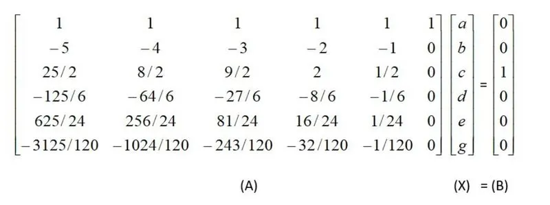
After solving the matrix we get the coefficients as
a=-0.83333
b=5.08333
c=-13.00000
d=17.83333
e=-12.83333
g=3.750000
Now dividing the hypothysis (1) by( Δx)^2 we get:
( ∂ˆ2 u/ ∂xˆ2 )=(a*f(i-5)+b*f(i-4)+c*f(i-3)+d*f(i-2)+e*f(i-1)+g*f(i)/( Δx)^2
or, ( ∂ˆ2 u/ ∂xˆ2 )=(-0.83333*f(i-5)+5.08333*f(i-4)-13.00000*f(i-3)+17.83333*f(i-2)-12.83333*f(i-1)+3.750000*f(i))/( Δx)^2
finding order of approximation:
Now again from the taylor equation we get
( ∂ˆ2 u/ ∂xˆ2 )=(a+b+c+d+e+g) *f(i)+(-5a-4b-3c-2d-e+0)f '(i) *(Δx)+(25a/2+8b+9c/2+2d+e/2+0)*f ''(i)*(Δx)^2+(-125a/6-64b/6-27c/6-8d/6-e/6+0)*f '''(i)*(Δx)^3+(625a/24+256b/24+81c/24+16d/24+e/24+0)f ''''(i)*(Δx)^4+(-3125a/120-1024b/120-243c/120-32d/120-e/120+0)*f '''''(i)*Δx)^5+(15625a/720+4096b/720+729c/720+64d/720+e/720+0)*f ''''''(i)*Δx)^6
on substituting the values of (i),(ii),(iii),(iv),(v) on the above equation we get:
( ∂ˆ2 u/ ∂xˆ2 )=(25a/2+8b+9c/2+2d+e/2+0)*f ''(i)*(Δx)^2+(15625a/720+4096b/720+729c/720+64d/720+e/720+0)*f ''''''(i)*Δx)^6
Dividing it by (Δx)^2 we get:
( ∂ˆ2 u/ ∂xˆ2 )=(25a/2+8b+9c/2+2d+e/2+0)*f ''(i)+(15625a/720+4096b/720+729c/720+64d/720+e/720+0)*f ''''''(i)*Δx)^4
In the above equation the value of (Δx)^4 is truncation error . As the order of truncation error is four so the equation is
fourth order approximation.
CODE TO COMPARE SECOND ORDER DERIVATIVE OFTHE FUNCTION EXP(X)*COS(X) WITH NUMARICAL APPROXIMATION THAT WE DERIVED ABOVE:
FUNCTION CODE:
CENTRAL DIFFERENCE ERROR:
function central_diff_error=centraldiff(x,dx)
%function=exp(x)*cos(x)
%f ''(x)=-2*exp(x)*sin(x)
analytical_derivative=-2*exp(x)*sin(x);
%numerical derivative
a=-0.083333;

b=1.333333;

c=-2.500000;

d=1.333333;

e=-.083333;
%central_diff_approx=(a*f(x-2*dx)+b*f(x-dx)+c*f(x)+d*f(x+dx)+e*f(x+2*dx))/(dx^2)
central_diff_approx=(a*(exp(x-2*dx)*cos(x-2*dx))+b*(exp(x-dx)*cos(x-dx))+c*(exp(x)*cos(x))+d*(exp(x+dx)*cos(x+dx))+e*(exp(x+2*dx)*cos(x+2*dx)))/(dx^2);

central_diff_error=abs(central_diff_approx-analytical_derivative)
left sided error:
function skewed_leftside_error=lefterror(x,dx)
%function=exp(x)*cos(x)
%f ''(x)=-2*exp(x)*sin(x)
analytical_derivative=-2*exp(x)*sin(x);
%numerical derivative
a=-0.83333;

b=5.08333;

c=-13.00000;

d=17.83333;

e=-12.83333;

g=3.750000;
% skewed left sided approx=(a*f(x-5*dx)+b*f(x-4*dx)+c*f(x-3*dx)+d*f(x-2*dx)+e*f(x-dx)+g*f(x))/(dx^2)
skewed_leftside_approx=(a*(exp(x-5*dx)*cos(x-5*dx))+b*(exp(x-4*dx)*cos(x-4*dx))+c*(exp(x-3*dx)*cos(x-3*dx))+d*(exp(x-2*dx)*cos(x-2*dx))+e*(exp(x-dx)*cos(x-dx))+g*(exp(x)*cos(x)))/(dx^2);
skewed_leftside_error=abs(skewed_leftside_approx-analytical_derivative)
RIGHT SIDED ERROR:
function skewed_rightsided_error=rightside(x,dx)
%function=exp(x)*cos(x)
%f ''(x)=-2*exp(x)*sin(x)
analytical_derivative=-2*exp(x)*sin(x);
%numerical derivative
a=3.75000;

b=-12.83333;

c=17.83333;

d=-13.00000;

e=5.08333;

g=-0.83333;
%skewed rightsided approx=a*f(x)+b*f(x+dx)+c*f(x+2*dx)+d*f(x+3*dx)+e*f(x+4*dx)+g*f(x+5*dx)
skewed_rightsided_approx=(a*(exp(x)*cos(x))+b*(exp(x+dx)*cos(x+dx))+c*(exp(x+2*dx)*cos(x+2*dx))+d*(exp(x+3*dx)*cos(x+3*dx))+e*(exp(x+4*dx)*cos(x+4*dx))+g*(exp(x+5*dx)*cos(x+5*dx)))/(dx^2);
skewed_rightsided_error=abs(skewed_rightsided_approx-analytical_derivative)
MAIN CODE:
clear all
close all
clc

x=pi/3;
dx=linspace(pi/4,pi/40000,40);
for i=1:length(dx)
    central_diff_error(i)=centraldiff(x,dx(i));
    skewed_leftside_error(i)=lefterror(x,dx(i));
    skewed_rightsided_error(i)=rightside(x,dx(i));
end
figure(1)
plot(dx,central_diff_error,"Color",'r','LineWidth',4)
hold on
plot(dx,skewed_leftside_error,"Color",'b','LineWidth',4)
plot(dx,skewed_rightsided_error,"Color",'g','LineWidth',4)
legend('central diff error','left sided error','right sided error')
grid on
xlabel('dx')
ylabel('error')
figure(2)
loglog(dx,central_diff_error,'color','r','linewidth',4)
hold on
loglog(dx,skewed_leftside_error,'color','b','LineWidth',4)
loglog(dx,skewed_rightsided_error,'color','g','linewidth',4)
legend('central diff error','left sided error','right sided error')
grid on
xlabel('dx')
ylabel('error')
RESULT:
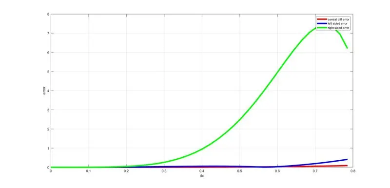
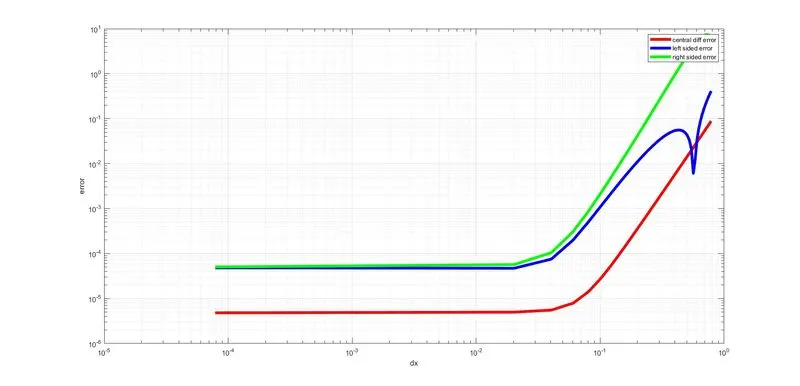
COMMAND WINDOW:
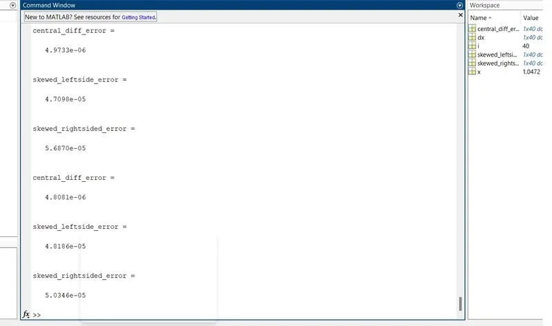
After analyzing dx vs error curve for central difference, left sided and right sided approximation we can conclude
that central difference value give more accurate or less error than left sided and right sided approximation.
In your own words, describe why a skewed scheme is useful? What can a skewed scheme do that a CD scheme cannot?
since we have noticed that central difference can give more accurate or less error than skewed schemes but
central difference scheme is not viable always. As for computing numerical approximation of a function at
corner or boundary condition we can not use central difference as it requires points from both side but for
skewed left or right points require at one side left or right.