Week 3.5 - Deriving 4th order approximation of a 2nd order derivative using Taylor Table method
AIM:- Deriving 4th order approximation of a 2nd order derivative using the Taylor Table method
OBJECTIVE:-
Derive the following 4th-order approximations of the second-order derivative.
1. Central difference
2. Skewed right-sided difference
3. Skewed left-sided difference
After deriving these schemes, prove that your skewed schemes are fourth-order accurate i.e the thumb rule given in
HINT (ii).:-
Once you have done this, write a program in Matlab to evaluate the second-order derivative of the analytical function exp(x)*cos(x) and compare it with the 3 numerical approximations that you have derived.
Provide a plot that compares the absolute error between the above-mentioned schemes
In your own words, describe why a skewed scheme is useful? What can a skewed scheme do that a CD scheme cannot?
HINT :
i) The order of accuracy P = Number of nodes in the stencil N - order of derivative Q + 1 for symmetric/central schemes
ii) The order of accuracy P = Number of nodes in the stencil N - order of derivative Q for one-sided/skewed schemes
iii) Solve the system of equations using the matrix inversion method in Matlab to obtain the Taylor table coefficients and use them directly in the numerical approximation statements to avoid input errors.
introduction:-
The differential equation is an equation.
which contains one or more terms that are in value derivative of the dependent variable.
An ordinary differential equation is one independent variable equation.
Q = -kAdT/dx.
dT = depend varible
dx = independent varible
ODE = Initial value problem
Partial diffrention Equation
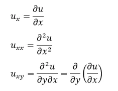
Partial differential equations are boundary value problems.
Discretization:-
in mathematics, discretization concerns the process of transferring continuous models and equations into discrete computer parts
This process is usually carried out as a first step toward making them suitable for numerical evaluation and implementation of a digital computer.
Different scheme:-
∂f/∂x, C. D. S . F. D. S. B. D. S.
Central Differencing Forward Differencing Backward Differencing
Scheme Scheme Scheme
Concept of stencil:-
In mathematics especially in the areas of numerical solutions of the partial differencing equation
Stencil is a generic arrangement of a node group that relates to the point of interest by using a numerical approximation routine.
Central differencing:- Here the nodes selected are symmetrical i.e. the data is taken from both sides of the point of focus.
Taylor's method, we get
∂f/∂x= af(i - 2) + b(i - 1) + cf(i) + df(i +2)
Here there are nodes taken from both sides of the point of focus i.e.(i).
(NOTE):- To select the number of nodes in consideration, we use the following expression:-
N = P+q -1 for central differencing
N = P + q for skewed differencing
Here N is no. of nodes, p is the order of derivative and q order of approximation.)
Taylor table for central difference:-
f(x) dx dx^2 dx^3 dx^4 d^5
f'(x) f''(x) f'''(x) f''''(x) f'''''(x)
af(i-1) a -2a 4a/2 -8a/6 16a/24 -32a/120
b(i-2) b -b b/2 -b/6 b/24 -b/120
cf(i) c 0 0 0 0 0
df(i-1) d d d/2 d/6 d/24 d/120
ef(i-2) e 2e 4e/2 8e/6 16e/24 32e/120
af(i-2) + bf(i-1)
+cf(i) +df(i+1)
+ef(i+2) 0 0 1 0 0 ?
it look at hypothetic term 1 to 5 term
This tabel transform into matrix of type Ax = B
a + b + c + d + e = 0 [1 1 1 1 1] [a] [0]
-2a - b + 0 + d + 2e = 0 [-2 -1, 0 1 2] [b] [0]
2a + b/2 + 0 + d/2 + 2e = 1 [ 2 1/2 0 1/2 2] [c] [0]
-8a/6 -b/6 + 0 + d/6 + 8e/6 = 0 [ 8/6 -1/6 0 1/6 8/6] [d] [0]
16/24 + b/24 + 0 + d/24 + 16e/24 =0 [ 16/24 1/24 0 1/24 16/24] [e] [0]
get the value of the unknown
i.e. values = a = -0.0833 b = 1.3333 c = 2.5000
d = 1.3333 e = 0.0833
These coefficients will further in code to get the value of derivative.
Skewed right sided difference:-
when the data point of the lift nodes are not aviable (at intial boundary conditions) .
we have to rely on the aviable data set
∂^2f/∂x^2 = af(i) + bf(i+1) +cf(1+i) + df(i+3) + ef(i+4) + ff(i+5)
Taylor's table for skewed right-sided differences
f(x) dxf'(x) dx^2f"(x) dx^3f'''(x) dx^4f''''(x) dx^5f'''''(x)
af(i) a 0 0 0 0 0
bf(i+1) b b b/2 b/6 b/24 b/120
cf(i+2) c 2c 4c/2 8c/6 16c/24 32c/120
df(i+3) d 3d 9d/2 27d/6 81d/24 243d/120
ef(i+4) e 4e 16e/2 64e/6 256e/24 1024e/120
ff(i+5) f 5f 25f/2 125f/6 625f/24 3125f/120
af(i)+bf(i+1)+
cf(i+2)+ df(i+3)
ef(i+4)+ff(i+5)
o 0 1 0 0 0
Tjis table transfer into matrix of the AX = B .
1 1 1 1 1 1 a 0
0 1 2 3 4 5 b 0
0 1/2 2 9/2 16/2 25/2 * c = 1
0 1/6 8/6 27/6 64/6 125/6 d 0
0 1/24 16/24 81/24 256/24 625/24 e 0
0 1/120 32/120 243/120 1024/120 3125/120 0
on further solving we get the value of the unkown values = a = 3.75000
b = -12.8333 c = 17.8333 d = 13.0000 e = 5.0833 f = 0.8333
These coefficients will futher used in code to set the value of derivative
Sekwed left sided difference.
When the data point of the left nodes is not available (at boundary conditions then we have to rely on the available data set).
∂^2f/∂x^2 = af(i - 5) + bf(i-4) + cf(i -3) + df(i-2) + ef(i-1)+ ff(i)
Taylor table for skewed right-sided difference
f(x) dxf(x) dx^2f''(x) dx^3f'''(x) dx^4f''''(x) dx^5f'''''(x)
af(i - 5) a -5a 25a/2 -125a/6 625a/24 3125a/120
bf(i-4) b -4b 16b/2 -64b/6 256b/24 -1024b/120
cf(i-3) c -3c 9c/2 -27c/6 81c/24 -243c/120
df(i-2) d -2d 4d/2 -8d/6 16d/24 -32d/120
ef(i-1) e -e e/2 e/6 e/24 -e/120
ff(i) f 0 0 0 0 0
af(i-5)+bf(i-4)+
cf(i-3) + df(i-2)+
ef(i-1)+ff(i)
0 0 1 0 0 0
This tabel tansform into matrix of type AX = B.
[ 1 1 1 1 1 1] a 0
[ -5 -4 -3 -2 -1 0] b 0
[ 25/2 16/2 9/2 2 1/2 0] * c = 1
[ -125/6 -64/6 -27/6 -8/6 -1/6 0] d 0
[ 625/24 256/24 81/24 16/24 7/24 0] e 0
[3121/120 -1o24/120 -243/120 32/120 1/120 0] f 0
unknown i.e. values = a= 0.8333 b = 5.08333 c = 13.0000 d = 17.8333 e = -12.8333
f = 3.7500
These coefficients will further use incode to get the value of derivative
step involved:-
1 we design the value of x and range of dx
2 we define an anonymous function of analytical function and its derivative.
3 use the matrices from the above-discussed section and solved it using the inversion method
i.e.
Ax = B = = X = A-1 B
And stored the coefficients in cf1 cf2 and cf3
4. Assigned the rows and columns to the appropriate matrices
5 . Loop the order of approximation expression in a for loop under the range of dx.
Here absolute error is also calculated from the derivative value calculated anal6ytically
6. The calculated values are plotted to do a better comparison
Matlab_code:-
clear all
close all

%analytical function defination and value assigment
x = pi/3;
dx = linspace (pi/10,pi/1000,100);
f = @(x)(exp(x)*cos(x));
g = @(x)(-2*exp(x)*sin(x));
d2f = g(x);
func = f(x);
%for central difference scheme.
%coefficient taken from taylor's table
 p = [1 1 1 1 1
    -2 -1 0 1 2
    4/2 1/2 0 1/2 4/2
    -8/6 -1/6 0 1/6 8/6
    16/24 1/24 0 1/24  16/24];
c = [0;0;1;0;0];
pc = inv(p)*c;
%as p*a = c i.e. a inverse (p)*c('fastest way to set by')
cf1 = pc;
%for right skewed difference scheme
q = [1 1 1 1 1 1
    0 1 2 3 4 5
    0 1/2 2 9/2 16/2 25/2
    0 1/6 8/6 27/6 64/6 125/6
    0 1/4 16/24 81/24 256/24 625/24
    0 1/120 32/120 243/120 1024/120 3125/120];
D = [0; 0; 1; 0; 0;0];
qD = inv(q)*D;
%as q*b = s i.e. b = inverse(q)*s (fastest way to get by")
cf2 = qD;
%for left skewed different scheme
R = [1 1 1 1 1 1
    -5 -4 -3 -2 -1 0
    25/2 16/2 9/2 2 1/2 0
    -125/6 -64/6 -27/6 -8/6 -1/6 0
    625/24  256/24  81/24  16/24  1/24 0
    -3125/120 -1024/120 -243/120 -32/120 -1/120 0];
E = [0; 0; 1; 0; 0; 0;];
RE = inv(R)*E;
%as n*b = s i.e. b = inverse(b)*s(fastest way to set by ")
cf3 = RE;
%calculated values of derivatives using C.D.S. R.S.D.C. L.S.D.C.
%defining variable size before using in loop
central_diff = zeros(1,100);
err_central = zeros(1,100);
right_sdiff = zeros(1,100);
err_right = zeros(1,100);
left_sdiff = zeros(1,100);
err_left = zeros(1,100);

for i = 1:length(dx)
    %calculating value and error by central difference scheme.
    central_diff(i) = (cf1(1)*f(x-2*dx(i))+ cf1(2)*f(x-dx(i))+cf1(3)*f(x)+cf1(4)*f(x+dx(i))+cf1(5)*f(x+2*dx(i)))/(dx(i))^2;
    err_central(i) = abs(central_diff(i)-d2f);

    %calculating value and error by right skewed difference scheme.
    right_sdiff(i) = (cf2(1)*f(x)+cf2(2)*f(x+dx(i))+cf2(3)*f(x+2*dx(i))+cf2(4)*f(x+3*dx(i))+ cf2(5)*f(x+4*dx(i))+cf2(6)*f(x+5*dx(i)))/(dx(i))^2;
    err_central(i) = abs(central_diff(i)-d2f);

    %calculating value and error by right skewed difference scheme
    %right_sdiff(i) = (cf2(1)*f(x)+ cf2(2)*f(x+dx(i))+cf2(3)*f(x+3*dx(i))+cf2(5)*f(x+4*dx(i))+cf2(6)*f(x+5*dx(i))/(dx(i))^2;
    %err_right(i) =abs(right_sdiff(i)-d2f);

    %calculate value and error by left skewed difference skewed.
    left_sdiff(i) = (cf3(1)*f(x-5*dx(i))+ cf3(2)*f(x-4*dx(i))+ cf3(3)*f(x-3*dx(i))+cf3(4)*f(x-2*dx(i))+ cf3(5)*f(x-dx(i))+cf3(6)*f(i))/dx(i)^2;
    err_left(i) = abs(left_sdiff(i)-d2f);
end
%plotting values of derivative
subplot (2,1,1)
hold on
fplot(d2f,'--')
xlim([-0.05 0.35]);
plot(dx,central_diff,'linewidth',2,'color','r');
plot(dx,central_diff,'linewidth',2,'color','g');
legend('analytical value at x = pi/3','central diff.',' right skewed diff.',' left skewed diff.','location','best')
xlabel('Grid siza(dx)');
ylabel('value');
title('comparision bw value of derivative calcuated by diff. order of approximation')
hold off
%plotting errors in approximatiion of derivative
subplot(2,1,2)
loglog(dx,err_central,'linewidth',2,'color','b');
hold on
xlim([.002 0.4]);
loglog(dx,err_right,'linewidth',2,'color','b');
loglog(dx,err_left,'linewidth',2,'color','g');
legend('cental diff.','right skewed diff.','left skewed diff.','location','best')
xlabel('grid siza(dx)');
ylabel('Absoulte error');
title('comparission b/w 4th order approximation method for error in calculating d2f/dx2');
Results:-
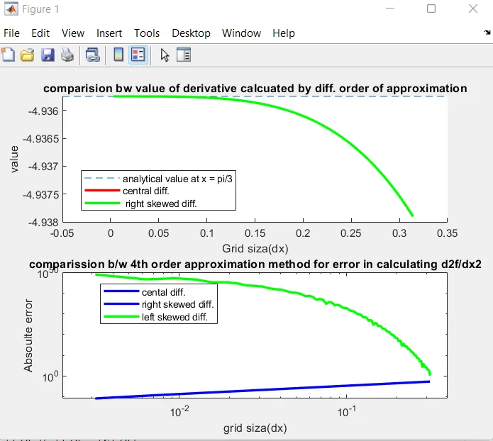
1 in the first plot we can see that the value of all the approximations approaches toward the analytically calculated value as the size of dx gets smaller.
2. on the second plot we can see that the error in the coefficient difference is lowest with respect to the other two