Week 3.5 - Deriving 4th order approximation of a 2nd order derivative using Taylor Table method

The objective of the report is to find the second-order derivative for the given function by using Central difference, Skewed right-sided differenc and Skewed left-sided difference of 4th order approximations.

FORMULAE - 

• The order of accuracy P = Number of nodes in the stencil N - order of derivative Q + 1 for symmetric/central schemes
• The order of accuracy P = Number of nodes in the stencil N - order of derivative Q   for one-sided/skewed schemes 

1) Central difference scheme -

    N = P+Q-1 = 4+2-1 = 5. So in the stencil for 4th order approximation symmetry schemes, 5 nodes values are required for computation.

let,

By solving the above equation with Taylor's table method, we get

2) Skewed right-sided difference scheme -

    N = P+Q = 4+2 = 6. So in the stencil for 4th order approximation skewed schemes, 6 nodes values are required for computation.

Let, 

By solving the above equation with Taylor's table method, we get

 

3) Skewed left-sided difference scheme -

    N = P+Q = 4+2 = 6. So in the stencil for 4th order approximation skewed schemes, 6 nodes values are required for computation.

Let, 

By solving the above equation with Taylor's table method, we get

CHECK, THE FORMULAE 2 IS CORRECT OR NOT 

In deriving the solution, the 6th and above order terms are neglected.

By expanding with taylor series, we get

(d2f/dx2) = (a+b+c+d+e+g)f(i) + (b+2c+3d+4e+5g)f'(i)dx + (b/2 + 4c/2 + 9d/2 + 16e/2 + 25g/2)f''(i)dx2 + (b/6 + 8c/6 + 27d/6 + 64e/6 + 125g/6)f'''(i)dx3 + (b/24 16c/24 + 81d/24 + 256e/24 + 625g/24)f''''(i)dx4 + (b/120 + 32c/120 + 243d/120 + 1024e/120 + 3125g/120)f'''''(i)dx5 + (b/720 + 64c/720 + 729d/720 + 4096e/720 + 15625g/720)f''''''(i)dx6

By simplification,we get

(d2f/dx2) = f''(i)/dx2 + 17.32f''''''(i)dx6/dx2 = f''(i)/dx2 + 17.32f''''''(i)dx4 = f''(i)/dx2 + O(dx4)

In the above equation, we are neglecting dx4 and above order terms, which indicates the method is 4th order approximation.

MATLAB CODE -

The Matlab code is attached below. 

function f = fun_value1(x,dx)
 f = exp(x+dx) * cos(x+dx);
end

clc;
clear all;
close all;

%f(x) = exp(x) * cos(x)
x = pi/3;
dx = linspace(1e-2,0.1,100);

for i=1:length(dx)
%Analytical solution second order derivative
analytical_sol(i) = exp(x)*(-2*sin(x));

%4th order approximation with second order derivative 
%1 - central scheme
central_scheme_sol(i) = ((-1/12)*fun_value1(x,-2*dx(i)) + (4/3)*fun_value1(x,-dx(i)) + (-5/2)*fun_value1(x,0) + (4/3)*fun_value1(x,dx(i)) + (-1/12)*fun_value1(x,2*dx(i)))/dx(i)^2 ;

%2 - right skewness
rightsided_scheme_sol(i) = ((15/4)*fun_value1(x,0) + (-77/6)*fun_value1(x,dx(i)) + (107/6)*fun_value1(x,2*dx(i)) + (-13)*fun_value1(x,3*dx(i)) + (61/12)*fun_value1(x,4*dx(i)) + (-5/6)*fun_value1(x,5*dx(i)))/dx(i)^2 ;

%3 - left skewness
leftsided_scheme_sol(i) = ((15/4)*fun_value1(x,0) + (-77/6)*fun_value1(x,-dx(i)) + (107/6)*fun_value1(x,-2*dx(i)) + (-13)*fun_value1(x,-3*dx(i)) + (61/12)*fun_value1(x,-4*dx(i)) + (-5/6)*fun_value1(x,-5*dx(i)))/dx(i)^2 ;

error_central_scheme(i) = abs(analytical_sol(i) - central_scheme_sol(i));
error_rightsided_scheme(i) = abs(analytical_sol(i) - rightsided_scheme_sol(i));
error_leftsided_scheme(i) = abs(analytical_sol(i) - leftsided_scheme_sol(i));

end

plot(dx,error_central_scheme)
hold on
plot(dx,error_rightsided_scheme)
hold on
plot(dx,error_leftsided_scheme,'-*')
xlabel('dx-value')
ylabel('error-value')
legend('central-scheme','rightsided-scheme','leftsided-scheme')

RESULTS - 

The second order derivate for the given function is calculated by using analytical and numerical methods. The fig 1 shows the errors obtained due to computing the derivative by central scheme, right-sided scheme, left-sided scheme by fourth order approximations. In the fig 1, it is observed that the central scheme gives accurate results compared to skewed schemes.

 

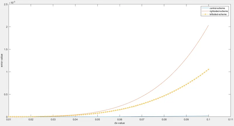
FIG 1 - dx V/S error value

In fig 1, it is observed that as the dx value increases, the error value increases in all 3 approximations. But, if dx value < 0.001, roundoff error is introduced which results in increase in the error as shown in fig 2.

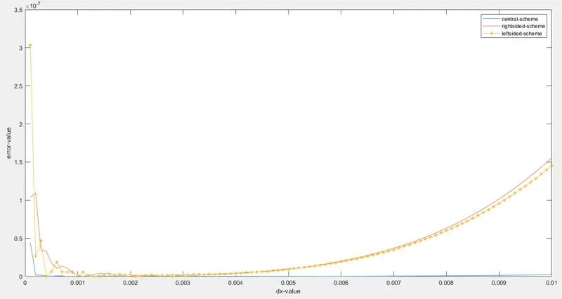
FIG 2 - ROUNDOFF ERROR

SKEWED SCHEME V/S CENTRAL SCHEME - 

From the fig1, it is observed that the central scheme shows accurate results compared to skewed schemes. But for the grid nodes at the domain boundaries, central scheme cannot calculate the results as it requires nodes present on both sides. So, in this situation skewed schemes are useful because in order to compute the results, it requires only one-sided nodes.