Week 3.5 - Deriving 4th order approximation of a 2nd order derivative using Taylor Table method

Aim:

The main aim is to derive the central difference, skewed right difference and skewed left difference scheme for the fourth-order approximation of the second-order derivative and creating the Taylor table.

Theory:

Central Differencing Scheme:

The central Difference scheme is a finite difference Method that optimizes the approximation for the differential operator in the central node of the considered patch and provides the numerical solutions to the differential equations.

For the central Differencing scheme, we need to know the number of nodes required to solve the derivative.

The number of nodes = p+q-1

Where, p= Order of the Derivative, q = Order of the Approximation

Therefore, the number of nodes = 2+4-1 = 5.

(Since we are calculating for the second-order derivative of the fourth-order approximation)

The second order derivative of the fourth-order approximation is

`∆x^2 (∂^2 f)/(∂x^2) =af(i-2)+bf(i-1)+cf(i)+df(i+1)+ef(i+2)`

Expanding the terms

`f(i-2)=f(i)-(f^' (i)(2∆x))/(1!)+f^'' (i)(2∆x)^2/(2!)-f^''' (i)(2∆x)^3/(3!)+f''''(i)(2∆x)^4/(4!)`

Multiply it with ‘a’

`a×f(i-2)=(a×f(i))-(a×f^' (i)(2∆x))/(1!)+(a×f^'' (i)(2∆x)^2)/(2!)-(a×f^''' (i)(2∆x)^3)/(3!)+(a×f^'''' (i)(2∆x)^4)/(4!)…(1)`

For `b×f(i-1)`

`b×f(i-1)=(b×f(i))-(b×f^' (i)(∆x))/(1!)+(b×f^'' (i)(∆x)^2)/(2!)-(b×f^''' (i)(∆x)^3)/(3!)+(b×f^'''' (i)(∆x)^4)/(4!)…(2)`

`c×f(i)=c×f(i)…(3)`

`d×f(i+1)=(d×f(i))+(d×f^' (i)(∆x))/(1!)+(d×f^'' (i)(∆x)^2)/(2!)+(d×f^''' (i)(∆x)^3)/(3!)+(d×f^'''' (i)(∆x)^4)/(4!)…(4)`

`e×f(i+2)=(e×f(i))+(e×f^' (i)(2∆x))/(1!)+(e×f^'' (i)(2∆x)^2)/(2!)+(e×f^''' (i)(2∆x)^3)/(3!)+(e×f^'''' (i)(2∆x)^4)/(4!)…(5)`

Here, we have five unknowns and therefore we get five equations and we can arrange the above equations in the Taylor Table.

Stencil	f(i)	`∆xf’(i)`	`∆x^2 f''(i)`	`∆x^3 f'''(i)`	`∆x^4 f''''(i)`
a. f(i-2)	a	-2a	2a	-4a/3	2a/3
b. f(i-1)	b	-b	b/2	-b/6	b/24
c. f(i)	c	0	0	0	0
d. f(i+1)	d	d	d/2	d/6	d/24
e. f(i+2)	e	2e	2e	4e/3	2e/3
	0	0	1	0	0

To solve the unknown a, b, c, d, and e values, we can either write a MATLAB code for it or we can manually calculate the values in the form of Matrix AX=B

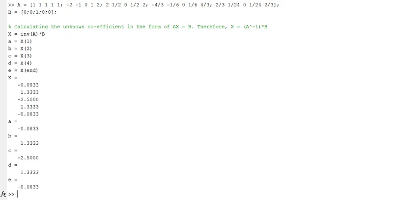
By Solving the Matrix in the MATLAB, we get.

a = -0.0833

b = 1.3333

c = -2.5000

d = 1.3333

e = -0.0833

Skewed Right-Sided Difference:

For the Skewed Right-Sided Difference scheme, we need to know the number of nodes required to solve the derivative.

The number of nodes = p+q-1

Where, p= Order of the Derivative, q = Order of the Approximation

Therefore, the number of nodes = 2+4-1 = 5.

(Since we are calculating for the second order derivative of the fourth-order approximation)

The second order derivative of the fourth-order approximation is

`∆x^2 (∂^2 f)/(∂x^2) =af(i)+bf(i+1)+cf(i+2)+df(i+3)+ef(i+4)+gf(i+5)`

Expanding the terms

`a×f(i)=a×f(i)…(1)`

`f(i+1)=f(i)+(f^' (i)(∆x))/1!+f^'' (i)(∆x)^2/(2!)+f^''' (i)(∆x) ^3/(3!)+f''''(i)(∆x)^4/(4!)+f^''''' (i)(∆x)^5/(5!)`

Multiply it with ‘a’

`b×f(i+1)=b×f(i)+(b×f^' (i)(∆x))/(1!)+(b×f^'' (i)(∆x)^2)/(2!)+(b×f^''' (i)(∆x)^3)/(3!)+(b×f''''(i)(∆x)^4)/(4!)+b×f^''''' (i)(∆x)^5/(5!)…(2)`

For `c×f(i+2)`

`c×f(i+2)=(c×f(i))+(c×f^' (i)(2∆x))/(1!)+(c×f^'' (i)(2∆x)^2)/(2!)+(c×f^''' (i)(2∆x)^3)/(3!)+c×f^'''' (i)(2∆x)^4/(4!)+c×f^''''' (i)(2∆x)^5/(5!)…(3)`

`d×f(i+3)=(d×f(i))+(d×f^' (i)(3∆x))/(1!)+(d×f^'' (i)(3∆x)^2)/(2!)+(d×f^''' (i)(3∆x)^3)/(3!)+d×f^'''' (i)(3∆x)^4/(4!)+d×f^''''' (i)(3∆x)^5/(5!)…(4)`

`e×f(i+4)=(e×f(i))+(e×f^' (i)(4∆x))/(1!)+(e×f^'' (i)(4∆x)^2)/(2!)+(e×f^''' (i)(4∆x)^3)/(3!)+e×f^'''' (i)(4∆x)^4/(4!)+e×f^''''' (i)(4∆x)^5/(5!)…(5)`

`g×f(i+5)=(g×f(i))+(g×f^' (i)(5∆x))/(1!)+(g×f^'' (i)(5∆x)^2)/(2!)+(g×f^''' (i)(5∆x)^3)/(3!)+g×f^'''' (i)(5∆x)^4/(4!)+g×f^''''' (i)(5∆x)^5/(5!)…(6)`

Here, we have five unknowns and therefore we get five equations and we can arrange the above equations in the Taylor Table.

Stencil	f(i)	`∆xf’(i)`	`∆x^2 f''(i)`	`∆x^3 f'''(i)`	`∆x^4 f''''(i)`	`∆x^5 f'''''(i)`
a. f(i)	a	0	0	0	0	0
b. f(i+1)	b	b	b/2	b/6	b/24	b/120
c. f(i+2)	c	2c	2c	4c/3	2e/3	32/120
d. f(i+3)	d	3d	9d/2	27d/6	81d/24	243d/120
e. f(i+4)	e	4e	8e	64e/6	256e/24	1024e/120
g.f(i+5)	g	5g	25g/2	125g/6	625g/24	3125g/120
	0	0	1	0	0	0

To solve the unknown a, b, c, d, and e values, we can either write a MATLAB code for it or we can manually calculate the values in the form of Matrix AX=B

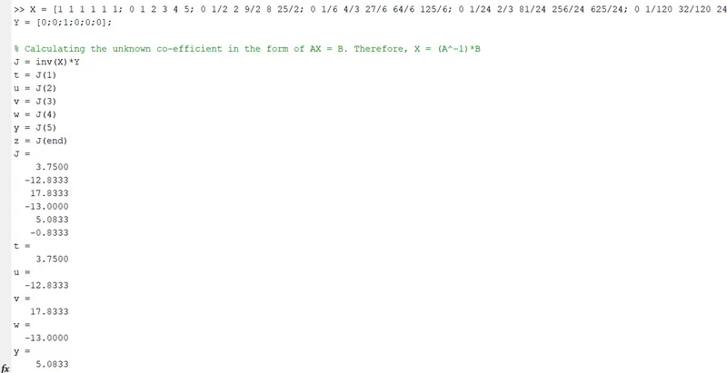
By Solving the Matrix in the MATLAB, we get.

a = 3.7500

b = -12.8333

c = 17.8333

d = -13.0000

e = 5.0833

g = -0.8333

Skewed Left Sided Difference:

For the Skewed left-Sided Difference scheme, we need to know the number of nodes required to solve the derivative.

The number of nodes = p+q-1

Where, p= Order of the Derivative, q = Order of the Approximation

Therefore, the number of nodes = 2+4-1 = 5.

(Since we are calculating for the second-order derivative of the fourth-order approximation)

The second-order derivative of the fourth-order approximation is

`∆x^2 (∂^2 f)/(∂x^2) =af(i)+bf(i+1)+cf(i+2)+df(i+3)+ef(i+4)+gf(i+5)`

Expanding the terms

`a×f(i-5)=(a×f(i))-(a×f^' (i)(5∆x))/(1!)+(a×f^'' (i)(5∆x)^2)/(2!)-(a×f^''' (i)(5∆x)^3)/(3!)+a×f^'''' (i)(5∆x)^4/(4!)-a×f^''''' (i)(5∆x)^5/(5!)…(1)`

`b×f(i-4)=(b×f(i))-(b×f^' (i)(4∆x))/(1!)+(b×f^'' (i)(4∆x)^2)/(2!)-(b×f^''' (i)(4∆x)^3)/(3!)+b×f^'''' (i)(4∆x)^4/(4!)-b×f^''''' (i)(4∆x)^5/(5!)…(2)`

`c×f(i-3)=(c×f(i))-(c×f^' (i)(3∆x))/(1!)+(c×f^'' (i)(3∆x)^2)/(2!)-(c×f^''' (i)(3∆x)^3)/(3!)+c×f^'''' (i)(3∆x)^4/(4!)-c×f^''''' (i)(3∆x)^5/(5!)…(3)`

`d×f(i-2)=(d×f(i))-(d×f^' (i)(2∆x))/(1!)+(d×f^'' (i)(2∆x)^2)/(2!)-(d×f^''' (i)(2∆x)^3)/(3!)+d×f^'''' (i)(2∆x)^4/(4!)-d×f^'''''(i)(2∆x)^5/(5!)…(4)`

`e×f(i-1)=(e×f(i))-(e×f^' (i)(∆x))/(1!)+(e×f^'' (i)(∆x)^2)/(2!)-(e×f^''' (i)(2∆x)^3)/(3!)+(e×f''''(i)(∆x)^4)/(4!)-e×f^''''' (i)(∆x)^5/(5!)…(5)`

`g×f(i)=g×f(i)…(6)`

Here, we have five unknowns and therefore we get five equations and we can arrange the above equations in the Taylor Table.

Stencil	f(i)	`∆x f'(i)`	`∆x^2 f''(i)`	`∆x^3 f'''(i)`	`∆x^4 f''''(i)`	`∆x^5 f'''''(i)`
a. f(i-5)	a	-5a	25a/2	-125a/6	625a/24	-3125a/120
b. f(i-4)	b	-4b	16b/2	-64b/6	256/24	-1024b/120
c. f(i-3)	c	-3c	9c/2	-27c/6	81e/24	-243/120
d. f(i-2)	d	-2d	4d/2	-8d/6	16d/24	-32d/120
e. f(i-1)	e	-e	e/2	-e/6	e/24	-e/120
g.f(i)	g	0	0	0	0	0
	0	0	1	0	0	0

To solve the unknown a, b, c, d, and e values, we can either write a MATLAB code for it or we can manually calculate the values in the form of Matrix AX=B

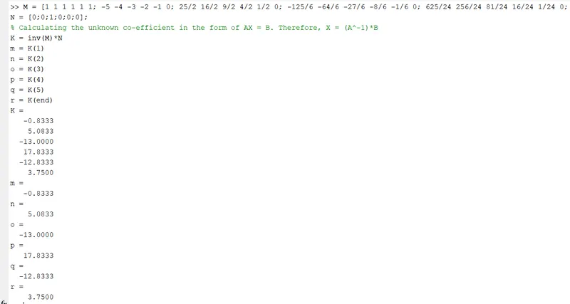
By Solving the Matrix in the MATLAB, we get.

a = -0.8333

b = 5.0833

c = -13.0000

d = 17.8333

e = -12.8333

g = 3.7500

Procedure:

To calculate the fourth-order approximation using the central differencing, Skewed Left side differencing and Skewed right side differencing, we need to substitute the above values in MATLAB to get the required output in the form of a graph.

• First, we need to enter the values of the ‘x’ and ‘dx’.

% Input Parameters
x = pi/3;
dx = linspace(pi/4,pi/400, 80);

• A for-loop is created to calculate the Error for the above-mentioned methods by subtracting the absolute value of the Numerical and Analytical Derivatives.

% A Loop to calculate the CDS, SRSD, SLSD in the range of dx.

for i = 1:length(dx)
    Central_difference_error(i) = central_differencing(x,dx(i));
    skewed_right_side_error(i) = Skewed_right_side_differencing(x,dx(i));
    skewed_left_side_error(i) = Skewed_left_side_differencing(x,dx(i));
    
end

• Next, the graph is plotted showing the ‘dx’ and the three different errors.
• Labels and legends are given to the plots and the model is saved in the same folder as the function.

% Plotting the Graphs
figure()
loglog(dx, Central_difference_error)
hold on
loglog(dx, skewed_right_side_error)
hold on 
loglog(dx, skewed_left_side_error)

xlabel('Step Size (dx)')
ylabel('Truncation Error')
legend('Central Difference', 'Skewed Right side', 'Skewed Left Side', 'location','Southeast')
saveas(gcf, 'Step size Vs Truncation Error.png')

Main Code:

Central Differencing function:

function CDS_error = central_differencing(x,dx)

% Analytical Function f(x) = exp(x)*cos(x)
% second order derivative is f''(x) = -2 exp(x)*sin(x)

df_double_dash_dt = -2*exp(x)*sin(x);

% Finding out Co-efficients for the Taylor Tabnle in CDS
A = [1 1 1 1 1; -2 -1 0 1 2; 2 1/2 0 1/2 2; -4/3 -1/6 0 1/6 4/3; 2/3 1/24 0 1/24 2/3];
B = [0;0;1;0;0];

% Calculating the unknown co-efficient in the form of AX = B. Therefore, X = (A^-1)*B 
X = inv(A)*B;
a = X(1);
b = X(2);
c = X(3);
d = X(4);
e = X(end);

% Numerical Derivative 
CDS_fourth_order_approx = ((a*exp(x-(2*dx))*cos(x-(2*dx)))+(b*exp(x-dx)*cos(x-dx))+(c*exp(x)*cos(x))+(d*exp(x+dx)*cos(x+dx))+(e*exp(x+(2*dx))*cos(x+(2*dx))))/(dx^2);

% Truncation Error 
CDS_error = abs(CDS_fourth_order_approx - df_double_dash_dt);
end

Skewed right side differencing function:

function SRSD_error = Skewed_right_side_differencing(x,dx)

% Analytical Function f(x) = exp(x)*cos(x)
% second order derivative is f''(x) = -2 exp(x)*sin(x)

df_double_dash_dt = -2*exp(x)*sin(x);

% Finding out Co-efficients for the Taylor Tabnle in CDS
X = [1 1 1 1 1 1; 0 1 2 3 4 5; 0 1/2 2 9/2 8 25/2; 0 1/6 4/3 27/6 64/6 125/6; 0 1/24 2/3 81/24 256/24 625/24; 0 1/120 32/120 243/120 1024/120 3125/120];
Y = [0;0;1;0;0;0];

% Calculating the unknown co-efficient in the form of AX = B. Therefore, X = (A^-1)*B 
J = inv(X)*Y;

t = J(1);
u = J(2);
v = J(3);
w = J(4);
y = J(5);
z = J(end);

% Numerical Derivative 
SRSD_fourth_order_approx = ((t*exp(x)*cos(x))+(u*exp(x+dx)*cos(x+dx))+(v*exp(x+(2*dx))*cos(x+(2*dx)))+(w*exp(x+(3*dx))*cos(x+(3*dx)))+(y*exp(x+(4*dx))*cos(x+(4*dx)))+(z*exp(x+(5*dx))*cos(x+(5*dx))))/(dx^2);

% Truncation Error 
SRSD_error = abs(SRSD_fourth_order_approx - df_double_dash_dt);
end

Skewed left side differencing function:

function SLSD_error = Skewed_left_side_differencing(x,dx)

% Analytical Function f(x) = exp(x)*cos(x)
% second order derivative is f''(x) = -2 exp(x)*sin(x)

df_double_dash_dt = -2*exp(x)*sin(x);

% Finding out Co-efficients for the Taylor Tabnle in CDS
M = [1 1 1 1 1 1; -5 -4 -3 -2 -1 0; 25/2 16/2 9/2 4/2 1/2 0; -125/6 -64/6 -27/6 -8/6 -1/6 0; 625/24 256/24 81/24 16/24 1/24 0; -3125/120 -1024/120 -243/120 -32/120 -1/120 0];
N = [0;0;1;0;0;0];

% Calculating the unknown co-efficient in the form of AX = B. Therefore, X = (A^-1)*B 
K = inv(M)*N;

m = K(1);
n = K(2);
o = K(3);
p = K(4);
q = K(5);
r = K(end);


%m = K(6);
%n = K(5);
%o = K(4);
%p = K(3);
%q = K(2);
%r = K(1);

% Numerical Derivative 
%SLSD_fourth_order_approx = ((m*exp(x)*cos(x))+(n*exp(x-dx)*cos(x-dx))+(o*exp(x-(2*dx))*cos(x-(2*dx)))+(p*exp(x-(3*dx))*cos(x-(3*dx)))+(q*exp(x-(4*dx))*cos(x-(4*dx)))+(r*exp(x-(5*dx))*cos(x-(5*dx))))/(dx^2);
SLSD_fourth_order_approx = ((m*exp(x-(5*dx))*cos(x-(5*dx)))+(n*exp(x-(4*dx))*cos(x-(4*dx)))+(o*exp(x-(3*dx))*cos(x-(3*dx)))+(p*exp(x-(2*dx))*cos(x-(2*dx)))+(q*exp(x-dx)*cos(x-dx))+(r*exp(x)*cos(x)))/(dx^2);
% Truncation Error 
SLSD_error = abs(SLSD_fourth_order_approx - df_double_dash_dt);
end

Main Program:

clear;clc;

% Input Parameters
x = pi/3;
dx = linspace(pi/4,pi/400, 80);


% A Loop to calculate the CDS, SRSD, SLSD in the range of dx.

for i = 1:length(dx)
    Central_difference_error(i) = central_differencing(x,dx(i));
    skewed_right_side_error(i) = Skewed_right_side_differencing(x,dx(i));
    skewed_left_side_error(i) = Skewed_left_side_differencing(x,dx(i));
    
end

% Plotting the Graphs
figure()
loglog(dx, Central_difference_error)
hold on
loglog(dx, skewed_right_side_error)
hold on 
loglog(dx, skewed_left_side_error)

xlabel('Step Size (dx)')
ylabel('Truncation Error')
legend('Central Difference', 'Skewed Right side', 'Skewed Left Side', 'location','Southeast')
saveas(gcf, 'Step size Vs Truncation Error.png')

Result:

It can be seen that the central difference has a low error compared to the Skewed right and left side difference. This is because central differencing takes the past and future approximations and thus it gives a stable output leading to less error.

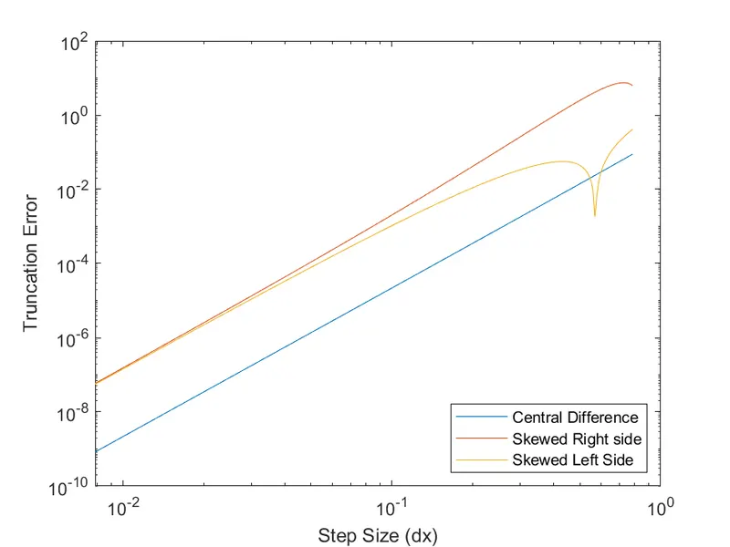
Describe why a skewed scheme is useful? What can a skewed scheme do that a CD scheme cannot?

A skewed scheme is used in the case where there is a boundary error calculation. Though the Error rate is higher in the skewed scheme compared to the central difference, it is manageable in the case of boundary error calculation.

The skewed scheme is used at the boundary where we cannot apply a central difference scheme as CDS takes the value from both ends. We can calculate the errors at boundary using forward difference or backward differencing but due to its low accuracy and therefore, a skewed scheme is used.