4th Order Approximation of a 2nd Order Derivative using Taylor Table Method
Taylor Series
The Taylor series of a function is an infinite sum of terms that are expressed in terms of the function's derivatives at a single point.
`f(x)=f(a)+(f'(a))/(1!)(x-a)+(f''(a))/(2!)(x-a)^2+(f'''(a))/(3!)(x-a)^3+...,`
For example, the below graph shows approximation at x=0, here we can see that as the number of terms increases the two curves becomes coincident.
The exponential function ex (in blue), and the sum of the first n + 1 terms of its Taylor series at 0 (in red).
Deriving the 4th order approximations of the second-order derivative
1) Skewed right-sided difference
The number of Nodes required for 4th order approximation of a second-order derivative can be given by the equation
`N=P+Q` where
`N` is the number of nodes
`Q` is the order of derivative
`P` is the order of approximation
So, here we need 6 nodes in order to find the 2nd order derivative with the 4th order of approximation.
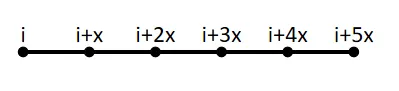
Consider the value of `(del^2y)/(delx^2)` with the 4th order of approximation is given by the equation
`(del^2y)/(delx^2)=af(i)+bf(i+1)+cf(i+2)+df(i+3)+ef(i+4)+gf(i+5)`
Now, using taylor series to find the values of discrete poits with repect to point `i`
`af(i)=af(i)`
`bf(i+1)=bf(i)+bDeltaxf'(i)+(bDeltax^2)/(2!)f''(i)+(bDeltax^3)/(3!)f'''(i)+(bDeltax^4)/(4!)f''''(i)+(bDeltax^5)/(5!)f'''''(i)+(bDeltax^6)/(6!)f''''''(i)+...`
`cf(i+2)=cf(i)+c(2Deltax)f'(i)+(c(2Deltax)^2)/(2!)f''(i)+(c(2Deltax)^3)/(3!)f'''(i)+(c(2Deltax)^4)/(4!)f''''(i)+(c(2Deltax)^5)/(5!)f'''''(i)+(c(2Deltax)^6)/(6!)f''''''(i)+...`
`df(i+3)=df(i)+d(3Deltax)f'(i)+(d(3Deltax)^2)/(2!)f''(i)+(d(3Deltax)^3)/(3!)f'''(i)+(d(3Deltax)^4)/(4!)f''''(i)+(d(3Deltax)^5)/(5!)f'''''(i)+(d(3Deltax)^6)/(6!)f''''''(i)+...`
`ef(i+4)=ef(i)+e(4Deltax)f'(i)+(e(4Deltax)^2)/(2!)f''(i)+(e(4Deltax)^3)/(3!)f'''(i)+(e(4Deltax)^4)/(4!)f''''(i)+(e(4Deltax)^5)/(5!)f'''''(i)+(e(4Deltax)^6)/(6!)f''''''(i)+...`
`gf(i+5)=gf(i)+g(5Deltax)f'(i)+g(5Deltax)^2/(2!)f''(i)+g(5Deltax)^3/(3!)f'''(i)+g(5Deltax)^4/(4!)f''''(i)+g(5Deltax)^5/(5!)f'''''(i)+g(5Deltax)^6/(6!)f''''''(i)+...`
Adding the LHS and RHS of the above equations we get
`af(i)+bf(i+1)+cf(i+2)+df(i+3)+ef(i+4)+gf(i+5)=f(i)[a+b+c+d+e+g]+Deltaxf'(i)[b+2c+3d+4e+5g]+Deltax^2f''(i)[b/2+(4c)/2+(9d)/2+(16e)/2+(25g)/2]+Deltax^3f'''(i)[b/6+(8c)/6+(27d)/6+(64e)/6+(125g)/6]+Deltax^4f''''(i)[b/24+(16c)/24+(81d)/24+(256e)/24+(625g)/24]+Deltax^5f'''''(i)[b/120+(32c)/120+(243d)/120+(1024e)/120+(3125g)/120]`
In the above equations, we want only the coefficients of `Deltax^2f''(i)` and we assume the coefficient to be one and for the remaining terms we assume the coefficients to be zero.
`a+b+c+d+e+g=0`
`b+2c+3d+4e+5g=0`
`b/2+(4c)/2+(9d)/2+(16e)/2+(25g)/2=1`
`b/6+(8c)/6+(27d)/6+(64e)/6+(125g)/6=0`
`b/24+(16c)/24+(81d)/24+(256e)/24+(625g)/24=0`
`b/120+(32c)/120+(243d)/120+(1024e)/120+(3125g)/120=0`
| Taylor Table | ||||||||
| Assumed Function | Taylor Series Expansion | |||||||
| `f(i)` | `Deltaf'(i)` | `Deltax^2f''(i)` | `Deltax^3f'''(i)` | `Deltax^4f''''(i)` | `Deltax^5f'''''(i)` | `Deltax^6f''''''(i)` | ||
|
Stencil
|
`af(i)` | `a` | `0` | `0` | `0` | `0` | `0` | `0` |
| `bf(i+1)` | `b` | `b` | `b/2` | `b/6` | `b/24` | `b/120` | `b/720` | |
| `cf(i+2)` | `c` | `2c` | `(4c)/2` | `(8c)/6` | `(16c)/24` | `(32c)/120` | `(64c)/720` | |
| `df(i+3)` | `d` | `3d` | `(9d)/2` | `(27d)/6` | `(81d)/24` | `(243d)/120` | `(729d)/720` | |
| `ef(i+4)` | `e` | `4e` | `(16e)/2` | `(64e)/6` | `(256e)/24` | `(1024e)/120` | `(4096e)720` | |
| `gf(i+5)` | `g` | `5g` | `(25g)/2` | `(125g)/6` | `(625g)/24` | `(3125g)/120` | `(15625g)/720` | |
| Sum of Coefficients | 0 | 0 | 1 | 0 | 0 | 0 | ? | |
Writing the coefficients in the form of a matrix we get
`[[1, 1, 1, 1, 1, 1],[0, 1, 2, 3, 4, 5],[0, 1/2, (4)/2, (9)/2, (16)/2, (25)/2],[0, 1/6, (8)/6, (27)/6, (64)/6, (125)/6],[0, 1/24, (16)/24, (81)/24, (256)/24, (625)/24],[0, 1/120, (32)/120, (243)/120, (1024)/120, (3125)/120]][[a],[b],[c],[d],[e],[g]]=[[0],[0],[1],[0],[0],[0]]`
Solving using MATLAB to find the values of the coefficients
>> A=[1 1 1 1 1 1;0 1 2 3 4 5;0 1/2 4/2 9/2 16/2 25/2;0 1/6 8/6 27/6 64/6 125/6;0 1/24 16/24 81/24 256/24 625/24;0 1/120 32/120 243/120 1024/120 3125/120]
B=[0;0;1;0;0;0]
X=AB

A =

    1.0000    1.0000    1.0000    1.0000    1.0000    1.0000
         0    1.0000    2.0000    3.0000    4.0000    5.0000
         0    0.5000    2.0000    4.5000    8.0000   12.5000
         0    0.1667    1.3333    4.5000   10.6667   20.8333
         0    0.0417    0.6667    3.3750   10.6667   26.0417
         0    0.0083    0.2667    2.0250    8.5333   26.0417


B =

     0
     0
     1
     0
     0
     0


X =

    3.7500
  -12.8333
   17.8333
  -13.0000
    5.0833
   -0.8333
Now we can write the equation using the Taylors Table as `(del^2y)/(delx^2)=(af(i)+bf(i+1)+cf(i+2)+df(i+3)+ef(i+4)+gf(i+5))/(Deltax^2)`
2) Skewed left-sided difference
The number of Nodes required for 4th order approximation of a second-order derivative can be given by the equation
`N=P+Q` where
`N` is the number of nodes
`Q` is the order of derivative
`P` is the order of approximation
So, here we need 6 nodes in order to find the 2nd order derivative with the 4th order of approximation.
Consider the value of `(del^2y)/(delx^2)` with the 4th order of approximation is given by the equation
`(del^2y)/(delx^2)=af(i)+bf(i-1)+cf(i-2)+df(i-3)+ef(i-4)+gf(i-5)`
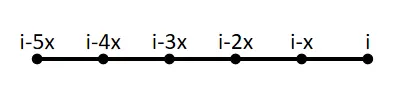
Consider Taylor Table for left-sided difference
| Taylor Table | ||||||||
| Assumed Function | Taylor Series Expansion | |||||||
| `f(i)` | `Deltaxf'(i)` | `Deltax^2f''(i)` | `Deltax^3f'''(i)` | `Deltax^4f''''(i)` | `Deltax^5f'''''(i)` | `Deltax^6f''''''(i)` | ||
|
Stencil
|
`af(i)` | `a` | `0` | `0` | `0` | `0` | `0` | `0` |
| `bf(i-1)` | `b` | `-b` | `b/2` | `-b/6` | `b/24` | `-b/120` | `b/720` | |
| `cf(i-2)` | `c` | `-2c` | `(4c)/2` | `-(8c)/6` | `(16c)/24` | `-(32c)/120` | `(64c)/720` | |
| `df(i-3)` | `d` | `-3d` | `(9d)/2` | `-(27d)/6` | `(81d)/24` | `-(243d)/120` | `(729d)/720` | |
| `ef(i-4)` | `e` | `-4e` | `(16e)/2` | `-(64e)/6` | `(256e)/24` | `-(1024e)/120` | `(4096e)720` | |
| `gf(i-5)` | `g` | `-5g` | `(25g)/2` | `-(125g)/6` | `(625g)/24` | `-(3125g)/120` | `(15625g)/720` | |
| Sum of Coefficients | 0 | 0 | 1 | 0 | 0 | 0 | ? | |
Writing the coefficients in the form of a matrix we get
`[[1, 1, 1, 1, 1, 1],[0, -1, -2, -3, -4, -5],[0, 1/2, (4)/2, (9)/2, (16)/2, (25)/2],[0, -1/6, -(8)/6, -(27)/6, -(64)/6, -(125)/6],[0, 1/24, (16)/24, (81)/24, (256)/24, (625)/24],[0, -1/120, -(32)/120, -(243)/120, -(1024)/120, -(3125)/120]][[a],[b],[c],[d],[e],[g]]=[[0],[0],[1],[0],[0],[0]]`
Solving using MATLAB to find the values of the coefficients
>> A=[1 1 1 1 1 1;0 -1 -2 -3 -4 -5;0 1/2 4/2 9/2 16/2 25/2;0 -1/6 -8/6 -27/6 -64/6 -125/6;0 1/24 16/24 81/24 256/24 625/24;0 -1/120 -32/120 -243/120 -1024/120 -3125/120]
B=[0;0;1;0;0;0]
X=AB

A =

    1.0000    1.0000    1.0000    1.0000    1.0000    1.0000
         0   -1.0000   -2.0000   -3.0000   -4.0000   -5.0000
         0    0.5000    2.0000    4.5000    8.0000   12.5000
         0   -0.1667   -1.3333   -4.5000  -10.6667  -20.8333
         0    0.0417    0.6667    3.3750   10.6667   26.0417
         0   -0.0083   -0.2667   -2.0250   -8.5333  -26.0417


B =

     0
     0
     1
     0
     0
     0


X =

    3.7500
  -12.8333
   17.8333
  -13.0000
    5.0833
   -0.8333
Now we can write the equation using the Taylors Table as `(del^2y)/(delx^2)=(af(i)+bf(i-1)+cf(i-2)+df(i-3)+ef(i-4)+gf(i-5))/(Deltax^2)`
3. Central Difference
The number of Nodes required for 4th order approximation of a second-order derivative can be given by the equation
`N=P+Q-1` where
`N` is the number of nodes
`Q` is the order of derivative
`P` is the order of approximation
So, here we need 5 nodes in order to find the 2nd order derivative with the 4th order of approximation.
Consider the value of `(del^2y)/(delx^2)` with the 4th order of approximation is given by the equation
`(del^2y)/(delx^2)=af(i-2)+bf(i-1)+cf(i)+df(i+1)+ef(i+2)`

Consider Taylor Table for central difference
| Taylor Table | |||||||
| Assumed Function | Taylor Series Expansion | ||||||
| `f(i)` | `Deltaxf'(i)` | `Deltax^2f''(i)` | `Deltax^3f'''(i)` | `Deltax^4f''''(i)` | `Deltax^5f'''''(i)` | ||
|
Stencil
|
`af(i-2)` | `a` | `-2a` | `(4a)/2` | `-(8a)/6` | `(16a)/24` | `-(32a)/120` |
| `bf(i-1)` | `b` | `-b` | `b/2` | `-b/6` | `b/24` | `-b/120` | |
| `cf(i)` | `c` | `0` | `0` | `0` | `0` | `0` | |
| `df(i+1)` | `d` | `d` | `d/2` | `d/6` | `d/24` | `-c/120` | |
| `ef(i+2)` | `e` | `2e` | `(4e)/2` | `-(8e)/6` | `(16e)/24` | `(32e)/120` | |
| Sum of Coefficients | 0 | 0 | 1 | 0 | 0 | ? | |
Writing the coefficients in the form of a matrix we get
`[[1, 1, 1, 1, 1],[-2, -1, 0, 1, 2],[4/2, 1/2, 0, 1/2, 4/2],[-8/6, -1/6, 0, 1/6, 8/6],[16/24, 1/24, 0, 1/24, 16/24],[-32/120, -1/120, 0, 1/120, 32/120]][[a],[b],[c],[d],[e]]=[[0],[0],[1],[0],[0]]`
Solving using MATLAB to find the values of the coefficients
>> A=[1, 1, 1, 1, 1;-2, -1, 0, 1, 2;4/2, 1/2, 0, 1/2, 4/2;-8/6, -1/6, 0, 1/6, 8/6;16/24, 1/24, 0, 1/24, 16/24]
B=[0;0;1;0;0]
X=AB

A =

    1.0000    1.0000    1.0000    1.0000    1.0000
   -2.0000   -1.0000         0    1.0000    2.0000
    2.0000    0.5000         0    0.5000    2.0000
   -1.3333   -0.1667         0    0.1667    1.3333
    0.6667    0.0417         0    0.0417    0.6667


B =

     0
     0
     1
     0
     0


X =

   -0.0833
    1.3333
   -2.5000
    1.3333
   -0.0833
Now we can write the equation using the Taylors Table as `(del^2y)/(delx^2)=(af(i-2)+bf(i-1)+cf(i)+df(i+1)+ef(i+2))/(Deltax^2)`
Inputs
The input here is the given function, `f(x)=e^xcosx`
The assumed inputs include the value of `x` and `dx`, the point where the function `f(x)` is defined and the grid spacing value `dx`. The value dx ranges form `pi/4000` to `1.5pi`. The analytical derivative of the function is found at the point `x`.
%analytical fucntion=(e^x)cos(x);

%analytical derivative
%f(x)=(e^x)cos(x)
%f'(x)=(e^x)cos(x)-(e^x)sin(x)=e^x[cosx-sinx]
%f''(x)=(e^x)cos(x)-(e^x)sin(x)-[(e^x)sin(x)+(e^x)cos(x)]
%f''(x)=-2*e^x*sin(x)

%given inputs
%given inputs
x=pi/3;     %derivative to be computed at x=pi/3
dx=linspace(pi/4000,1.5*pi,2000);   %grid spacing dx=(pi*(4000-1.5))/(4000*2000)

%analytical derivative
analytical_derivative=-2*exp(x)*sin(x);
Finding the coefficients and designing the anonyms fucntion
An anonyms function f(x)=e^xcosx is defined to compute the value to f(x) upon taking the value of x as input.
The coefficients of the assumed equation of the 2nd order derivative for each differencing technique is calculated and stored.
%creating Anonymous Function
f=@(x) exp(x)*cos(x);

%Skewed right-sided(4th order approimation)
%Solving for the coefficients
A=[1 1 1 1 1 1;0 1 2 3 4 5;0 1/2 4/2 9/2 16/2 25/2;0 1/6 8/6 27/6 64/6 125/6;0 1/24 16/24 81/24 256/24 625/24;0 1/120 32/120 243/120 1024/120 3125/120];
B=[0;0;1;0;0;0];
x_r=AB;

%Skewed left-sided(4th order approimation)
%Solving for the coefficients
C=[1 1 1 1 1 1;0 -1 -2 -3 -4 -5;0 1/2 4/2 9/2 16/2 25/2;0 -1/6 -8/6 -27/6 -64/6 -125/6;0 1/24 16/24 81/24 256/24 625/24;0 -1/120 -32/120 -243/120 -1024/120 -3125/120];
D=[0;0;1;0;0;0];
x_l=CD;

%central differencing(4th order approimation)
%Solving for the coefficients
E=[1, 1, 1, 1, 1;-2, -1, 0, 1, 2;4/2, 1/2, 0, 1/2, 4/2;-8/6, -1/6, 0, 1/6, 8/6;16/24, 1/24, 0, 1/24, 16/24];
F=[0;0;1;0;0];
x_c=EF;
Numerical Derivative
A for loop is formulated to calculate the numerical derivative of the function using the assumed equation and found coefficients. For loops runs for every value of dx and the loop indexing is used to store the values at respective indexes.
The value of the numerical derivative is compared with the analytical derivative to find the absolute error.
for i=1:length(dx)

%numerical derivative

%Skewed right-sided(4th order approimation)
%f''(x)=af(i)+bf(i+1)+cf(i+2)+df(i+3)+ef(i+4)+gf(i+5)
nd_right_difference(i)=(x_r(1)*f(x)+x_r(2)*f(x+dx(i))+x_r(3)*f(x+2*dx(i))+x_r(4)*f(x+3*dx(i))+x_r(5)*f(x+4*dx(i))+x_r(6)*f(x+5*dx(i)))/(dx(i)^2);

%Skewed left-sided(4th order approimation)
%f''(x)=af(i)+bf(i-1)+cf(i-2)+df(i-3)+ef(i-4)+gf(i-5)
nd_left_difference(i)=(x_l(1)*f(x)+x_l(2)*f(x-dx(i))+x_l(3)*f(x-2*dx(i))+x_l(4)*f(x-3*dx(i))+x_l(5)*f(x-4*dx(i))+x_l(6)*f(x-5*dx(i)))/(dx(i)^2);

%central differencing(4th order approimation)
%f''(x)=af(i-2)+bf(i-1)+cf(i)+df(i+1)+ef(i+2)
nd_cent_difference(i)=(x_c(1)*f(x-2*dx(i))+x_c(2)*f(x-1*dx(i))+x_c(3)*f(x)+x_c(4)*f(x+dx(i))+x_c(5)*f(x+2*dx(i)))/(dx(i)^2);

%absolute error at x = pi/3
error_r(i)=abs(analytical_derivative-nd_right_difference(i));
error_l(i)=abs(analytical_derivative-nd_left_difference(i));
error_c(i)=abs(analytical_derivative-nd_cent_difference(i));
error=[error_r;error_l;error_c];

end
Plotting the function
To the error comparison for the three methods, we use the function 'loglog' with the 'absolute error' on the y-axis and the 'dx' on the x-axis, and we use the respective functions title, label and legend for annotating the plot
%Plotting the Absolute Error Curves
figure(1)
loglog(dx,error_r) %Plot both the axis on the log scale
grid on
hold on
loglog(dx,error_l)
loglog(dx,error_c)
ylabel('Absolute Error (Log Scale)')
xlabel('Grid Spacing (dx in Log Scale)')
legend('Right Differencing','Left Differencing','Central Differencing')
title('Absolute Error Comparison')
Complete Code
clear all
close all
clc

%analytical fucntion=(e^x)cos(x);

%analytical derivative
%f(x)=(e^x)cos(x)
%f'(x)=(e^x)cos(x)-(e^x)sin(x)=e^x[cosx-sinx]
%f''(x)=(e^x)cos(x)-(e^x)sin(x)-[(e^x)sin(x)+(e^x)cos(x)]
%f''(x)=-2*e^x*sin(x)

%given inputs
%given inputs
x=pi/3;     %derivative to be computed at x=pi/3
dx=linspace(pi/4000,1.5*pi,2000);   %grid spacing dx=(pi*(4000-1.5))/(4000*2000)

%analytical derivative
analytical_derivative=-2*exp(x)*sin(x);

%creating Anonymous Function
f=@(x) exp(x)*cos(x);

%Skewed right-sided(4th order approimation)
%Solving for the coefficients
A=[1 1 1 1 1 1;0 1 2 3 4 5;0 1/2 4/2 9/2 16/2 25/2;0 1/6 8/6 27/6 64/6 125/6;0 1/24 16/24 81/24 256/24 625/24;0 1/120 32/120 243/120 1024/120 3125/120];
B=[0;0;1;0;0;0];
x_r=AB;

%Skewed left-sided(4th order approimation)
%Solving for the coefficients
C=[1 1 1 1 1 1;0 -1 -2 -3 -4 -5;0 1/2 4/2 9/2 16/2 25/2;0 -1/6 -8/6 -27/6 -64/6 -125/6;0 1/24 16/24 81/24 256/24 625/24;0 -1/120 -32/120 -243/120 -1024/120 -3125/120];
D=[0;0;1;0;0;0];
x_l=CD;

%central differencing(4th order approimation)
%Solving for the coefficients
E=[1, 1, 1, 1, 1;-2, -1, 0, 1, 2;4/2, 1/2, 0, 1/2, 4/2;-8/6, -1/6, 0, 1/6, 8/6;16/24, 1/24, 0, 1/24, 16/24];
F=[0;0;1;0;0];
x_c=EF;

for i=1:length(dx)

%numerical derivative

%Skewed right-sided(4th order approimation)
%f''(x)=af(i)+bf(i+1)+cf(i+2)+df(i+3)+ef(i+4)+gf(i+5)
nd_right_difference(i)=(x_r(1)*f(x)+x_r(2)*f(x+dx(i))+x_r(3)*f(x+2*dx(i))+x_r(4)*f(x+3*dx(i))+x_r(5)*f(x+4*dx(i))+x_r(6)*f(x+5*dx(i)))/(dx(i)^2);

%Skewed left-sided(4th order approimation)
%f''(x)=af(i)+bf(i-1)+cf(i-2)+df(i-3)+ef(i-4)+gf(i-5)
nd_left_difference(i)=(x_l(1)*f(x)+x_l(2)*f(x-dx(i))+x_l(3)*f(x-2*dx(i))+x_l(4)*f(x-3*dx(i))+x_l(5)*f(x-4*dx(i))+x_l(6)*f(x-5*dx(i)))/(dx(i)^2);

%central differencing(4th order approimation)
%f''(x)=af(i-2)+bf(i-1)+cf(i)+df(i+1)+ef(i+2)
nd_cent_difference(i)=(x_c(1)*f(x-2*dx(i))+x_c(2)*f(x-1*dx(i))+x_c(3)*f(x)+x_c(4)*f(x+dx(i))+x_c(5)*f(x+2*dx(i)))/(dx(i)^2);

%absolute error at x = pi/3
error_r(i)=abs(analytical_derivative-nd_right_difference(i));
error_l(i)=abs(analytical_derivative-nd_left_difference(i));
error_c(i)=abs(analytical_derivative-nd_cent_difference(i));
error=[error_r;error_l;error_c];

end

%Plotting the Absolute Error Curves
figure(1)
loglog(dx,error_r) %Plot both the axis on the log scale
grid on
hold on
loglog(dx,error_l)
loglog(dx,error_c)
ylabel('Absolute Error (Log Scale)')
xlabel('Grid Spacing (dx in Log Scale)')
legend('Right Differencing','Left Differencing','Central Differencing')
title('Absolute Error Comparison')
Results
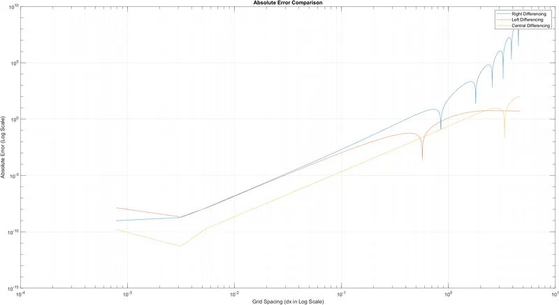
The comparison of absolute error for the left, right and central differencing scheme can be seen in the below graph. The graph shows that the central scheme is most accurate compared to the skewed differencing. The curves also show that when the value of dx is very small or large the approximating function becomes unstable. This instability is caused due to the combination of various errors such as roundoff error, residual error and truncation error.
From the below graph it is seen that the range of dx where the function is stable ranges from 0.1 to 0.01, beyond this range we see an abrupt rise or fall.
Q. Why skewed scheme is useful? What can a skewed scheme do that a central differencing scheme cannot?
A skewed scheme is useful when we have to predict using the boundary condition as we have only one direction to go. Hence the skewed scheme will be useful and we cannot use the central differencing scheme for such an application because it required information from both directions of the point.