Week 3.5 - Deriving 4th order approximation of a 2nd order derivative using Taylor Table method

Aim:-

To derive the following 4th order approximations of the second-order derivative of a function `f(x)=e^x×cos(x)` and compare the result with three numerical discretization schemes as stated

1. Central difference

2. Skewed right-sided difference

3. Skewed left-sided difference

Writing a matlab code to derive the analytical function and then comparing the absolute error between three defined schemes.

Theory:-

Discretization is the way through which we can convert the partial differential equation to algebra form by using taylor table

Taylar series is stated as Taylar expansion series

`f(x+∆x)= f(x)+∂f/∂x ∆x+(∂^2 f)/(∂x^2 ) (∆x)^2/2!+(∂^3 f)/(∂x^3 ) (∆x)^3/3!+⋯++(∂^n f)/(∂x^n ) (∆x)^n/n!`

For deriving the higher order approximations, it is not as simple to just apply some algebraic operation and
get the results but rather it becomes too complex to convert derivate into algebraic equations.
To ease out, we use a handy tool called as ‘Taylor Table’ to derive. The process starts with assuming a
polynomial based on terms i.e. grid points which depends on an order of approximation and derivative. The
coefficients of polynomial are unknowns which are inserted into the Taylor table and evaluation done either
through simple manipulation or matrix calculation.We can use the above defined three schems for computing 4th order approximation of the second order derivative

(1) Central differencing scheme

Let us consider 5 grid points including x as central grid point, i.e.

`(x-2Δx),(x- Δx),(x),(x+Δx),and (x+2Δx)`

and form a taylor table for solving the coefficient.

Based on selected grid points, a polynomial is assumed shown below.

`(∂^2 f)/(∂x^2 )=a.f(x-2∆x)+b.f(x-∆x)+c.f(x)+d.f(x+∆x)+e.f(x+2∆x)`

for each of the grid point function we have to form a taylor series then put the coefficient in taylor table as shown below

i+2 is 2`Δx`way from the the i . so by this way we form ore table series.

So, on coupling together terms to form equations

a + b + c + d + e = 0
−2a − b + d + 2e = 0
4a + b + d + 4e = 1 × 2!
−8a − b + d + 8e = 0
16a + b + d + 16e = 0

Above algebraic equations written into matrix form,

by solving the matrix, we have five unknown and five equation,we are not going to sixith equation.but we know the the second order derivative coefficient equals to one and we dont know is it same for sixth also because it do not eleiminated.

then by substituting to our seond order and sixth order term we get

`f^'' (x).(∆x)^2+((64a+b+d+64e))/(6!) f^(vi) (x).(∆x)^6`

Since, pairs (a, e) and (b, d) are equal. The sixth derivative doesn’t get eliminated.On further equating with polynomial and dividing both sides with`(∆x)^2`

`(-f(x-2∆x)+16.f(x-∆x)-30.f(x)+16.f(x+∆x)-f(x+2∆x))/(12(∆x)^2 ) =f^(2) (x)+O(∆x)^4`

`0(∆x)^4`represents the truncation error of fourth order approximation.

Hence, we have derived the fourth order central difference approximation scheme of second order derivative mentioned below.

`(∂^2 f)/(∂x^2 )≈(-f(x-2∆x)+16.f(x-∆x)-30.f(x)+16.f(x+∆x)-f(x+2∆x))/(12(∆x)^2 )`

(2) Skewed right-sided difference

Let us consider 5 grid points including x as leftmost grid point, i.e.

`(x), (x + Δx), (x + 2Δx), (x + 3Δx), and (x + 4Δx)`

Based on selected grid points, a polynomial is assumed shown below.

`(∂^2 f)/(∂x^2 )=a.f(x)+b.f(x+∆x)+c.f(x+2∆x)+d.f(x+3∆x)+e.f(x+4∆x)`

So, on coupling together terms to form equations

a + b + c + d + e = 0
b + 2c + 3d + 4e = 0
b + 4c + 9d + 16e = 1 × 2!
b + 8c + 27d + 64e = 0
b + 16c + 81d + 256e = 0

Above algebraic equations written into matrix form,

On solving matrix,

On substituting,

`f^2 (x).(∆x)^2+((b+64c+729d+4096e))/(6!) f^(vi) (x).(∆x)^6`

Since, pairs (a, e) and (b, d) are equal. The sixth derivative doesn’t get eliminated.On further equating with polynomial and dividing both sides with `(∆x)^2``

`(35.f(x)-104.f(x+∆x)+114.f(x+2∆x)-56.f(x+3∆x)+11.f(x+4∆x))/(12(∆x)^2 ) =f^2 (x)+O(∆x)^4`

`0(∆x)^4` represents the truncation error of fourth order approximation.
Hence, we have derived the fourth order skewed right sided difference approximation scheme of second order derivative mentioned below:

`(∂^2 f)/(∂x^2 )≈(35.f(x)-104.f(x+∆x)+114.f(x+2∆x)-56.f(x+3∆x)+11.f(x+4∆x))/(12(∆x)^2 )`

(3) Skewed left-sided difference

Let us consider 5 grid points including x as rightmost grid point, i.e.

`(x − 4Δx), (x − 3Δx), (x − 2Δx), (x − Δx), and (x)`

Based on selected grid points, a polynomial is assumed shown below.

`(∂^2 f)/(∂x^2 )=a.f(x)+b.f(x-∆x)+c.f(x-2∆x)+d.f(x-3∆x)+e.f(x-4∆x)`

So, on coupling together terms to form equations and reversing sign for equations (2) and (4).
Results in same set of equations as obtained in previous section (skewed right-sided difference scheme):

a + b + c + d + e = 0
b + 2c + 3d + 4e = 0
b + 4c + 9d + 16e = 1 × 2!
b + 8c + 27d + 64e = 0
b + 16c + 81d + 256e = 0

On solving,

On substituting,

`f^2 (x).(∆x)^2+((b+64c+729d+4096e))/(6!) f^(vi) (x).(∆x)^6`

Since, pairs (a, e) and (b, d) are equal. The sixth derivative doesn’t get eliminated.On further equating with polynomial and dividing both sides with `(∆x)^2`

`(35.f(x)-104.f(x-∆x)+114.f(x-2∆x)-56.f(x-3∆x)+11.f(x-4∆x))/(12(∆x)^2 ) =f^2 (x)+O(∆x)^4`

`0(∆x)^4` represents the truncation error of fourth order approximation.
Hence, we have derived the fourth order skewed left sided difference approximation scheme of second
order derivative mentioned below:

`(∂^2 f)/(∂x^2 )≈(35.f(x)-104.f(x-∆x)+114.f(x-2∆x)-56.f(x-3∆x)+11.f(x-4∆x))/(12(∆x)^2 )`

Actual function we are differentiating is `f(x)=e^x×cos(x)` and its second order derivative is `(∂^2 f)/(∂x^2 )=-2×e^x×sin⁡(x)`

The exact 2nd order derivative is obtained at ‘pi/3’. While, approximate values of 2nd order derivative is

obtained by different schemes mentioned below and compared with exact solution.

The computed absolute error is plotted based on discretization for different 4th order scheme. To be much
clearer about the different schemes, the consistency plot is obtained which helps us to understand which
scheme is better w.r.t slope of respective schemes.

Solution:-

Matlab code for our problem is

defined sub fuctions

1) "fourth_order"

function out=fourth_order(x)
out=exp(x)*cos(x);
end

2) "scheme"

function out=scheme(gp,dx)
% central differencing of 4th order approximation
central_order4=(-gp(3)+16*gp(4)-30*gp(5)+16*gp(6)-gp(7))/(12*(dx^2));
% skewed right side differencing of 4th order approximation
skewed_right4=(35*gp(5)-104*gp(6)+114*gp(7)-56*gp(8)+11*gp(9))/(12*(dx^2));
% skewed left side differencing of 4th order approximation
skewed_left4=(35*gp(5)-104*gp(4)+114*gp(3)-56*gp(2)+11*gp(1))/(12*(dx^2));
out=[central_order4 skewed_right4 skewed_left4];
end

3) "main_program"

clear all
close all
clc
% input varible
x=pi/3;
%discretization of function for range of dx
dx=linspace(pi/15,pi/400,50);
%analatical solution of second derivative of function
%f"(x)=-2*exp(x)*sin(x)
actual_solution=-2*exp(x)*sin(x);
for m=1:length(dx)
    % evaluating function at all 9 grid points from i-4 to i+4 
    for j=1:9
        gp(j)=fourth_order(x+((j-5)*dx(m)));
    end
    % 4th order approx for computing second order derivative
    deriv_order4(m,:)=scheme(gp,dx(m));
end
% absolute error value for each of the above applied schemes
error=abs(actual_solution-deriv_order4);
% plotting the absolute error

% plot of absolute error VS dx
figure(1)
loglog(dx,error(:,1),'color','b','marker','D');
hold on
loglog(dx,error(:,2),'color','g','marker','s');
loglog(dx,error(:,3),'color','r','marker','o');
title('Variation of absolute error based on discretization at different scheme');
xlabel('dx');
ylabel('Absolute error');
legend('Central differencing of 4th order ','Skewed right side differnce of 4th order','Skewed right side differnce of 4th order');

A plot shown in figure 1, show the comparison of 4th Order Schemes for Second Order Derivative

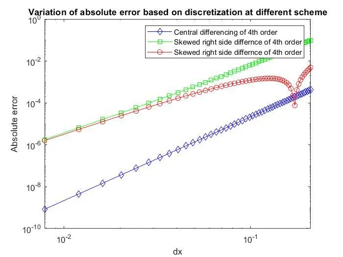
Figure 1, comparison plot

It can be observed that the central difference scheme would yield lower absolute error in comparison to other two schemes. It also approaches to zero absolute error at much higher rate. Thus, it must be preferred amongst the three 4th order scheme.
Through the skewed left sided scheme plot, it can be seen that initially absolute error tends to reduce at much higher rate. As the ‘dx’ is reduced, the sudden increase in absolute error is observed and then reduction in absolute error at slower rate.

Schewed scheme:-

The word skew means to be biased. Suppose, if the bulk of grid points are towards the right of the reference
grid point, then it is said to be positively skewed or skewed right-sided scheme. But, if the bulk of grid points
are towards the left of the reference grid point, then it is said to be negatively skewed or skewed left-sided
scheme. Same thing could be observed and said regarding the forward and backward differencing scheme
irrespective of only two grid points used to evaluate the first order derivative.

as we have already deine the 9 grid point to define stensile for both skewed scheme left and right

For skewed right scheme `(∂^2 f)/(∂x^2 )≈(35.f(x)-104.f(x+∆x)+114.f(x+2∆x)-56.f(x+3∆x)+11.f(x+4∆x))/(12(∆x)^2 )`

For skewed left scheme `(∂^2 f)/(∂x^2 )≈(35.f(x)-104.f(x-∆x)+114.f(x-2∆x)-56.f(x-3∆x)+11.f(x-4∆x))/(12(∆x)^2 )`

On observing above two schemes, we can say that the coefficient of function at particular pairs of grid point are same. These pairs can be (0, 0), (-1, +1), (-2, +2), (-3, +3), ... and so on depending on the scheme. Thus, any skewed scheme can be applied anywhere in the grid in the form as either left-sided or right-sided scheme.

Advantages of Skewed Scheme over Central Differencing Scheme:-

In order to apply approximation scheme at boundaries, only skewed schemes are applicable. While due to unavailability of grid points on one of the sides of the boundary, central difference scheme can’t be applied. Because, CDS requires number of grid points on both sides of the reference points depending on the order of the approximation scheme and order of derivative to be evaluated.