Week 3.5 - Deriving 4th order approximation of a 2nd order derivative using Taylor Table method

Derive the following 4th order approximations of the second-order derivative.

1. Central difference
2. Skewed right-sided difference
3. Skewed left-sided difference

After deriving these schemes, prove that your skewed schemes are fourth-order accurate i.e the thumb rule given in HINT (ii).

Once you have done this, write a program in Matlab to evaluate the second-order derivative of the analytical function exp(x)*cos(x) and compare it with the 3 numerical approximations that you have derived.

Provide a plot that compares the absolute error between the above-mentioned schemes

In your own words, describe why a skewed scheme is useful? What can a skewed scheme do that a CD scheme cannot?

HINT :

1. i) The order of accuracy P= Number of nodes in the stencil N- order of derivative Q + 1 for symmetric/central schemes
2. ii) The order of accuracy P= Number of nodes in the stencil N- order of derivative Q for one-sided/skewed schemes

iii) Solve the system of equations using the matrix inversion method in Matlab to obtain the taylor table coefficients and use them directly in the numerical approximation statements to avoid input errors.

Solution:- Given Function:-

`f(x) = exp(x)*cos(x)`

`f’’(x) = -2*exp(x)*sin(x)`

Central difference

Number of nodes = p+q-1

Number of nodes = 5

For Central differencing we can write

`(del^2f)/(delx^2) = a*f_(i-2) + b* f_(i-1) + c* f_(i) + d* f_(i+1) + e* f_(i+2)`

Since,

`a*f_(i-2) = a*[f_i - (2*Deltax)/(1!) * f'_i + (2*Deltax)^2/(2!) * f”_i - (2*Deltax)^3/(3!) * f'”_i + (2*Deltax)^4/(4!) * f_i^('v) - (2*Deltax)^5/(5!) * f_i^(v)]`

`b*f_(i-1) = [f_i - (Deltax)/(1!) * f'_i + (Deltax)^2/(2!) * f”_i - (Deltax)^3/(3!) * f'”_i + (Deltax)^4/(4!) * f_i^('v) - (Deltax)^5/(5!) * f_i^(v)]`

`c*f_i = c*f_i`

`d*f_(i+1) = d*[f_i + (Deltax)/(1!) * f'_i + (Deltax)^2/(2!) * f”_i + (Deltax)^3/(3!) * f'”_i + (Deltax)^4/(4!) * f_i^('v) + (Deltax)^5/(5!) * f_i^(v)]`

`e*f_(i+2) = e*[f_i + (2*Deltax)/(1!) * f'_i + (2*Deltax)^2/(2!) * f”_i + (2*Deltax)^3/(3!) * f'”_i + (2*Deltax)^4/(4!) * f_i^('v) + (2*Deltax)^5/(5!) * f_i^(v)]`

Now we can write as

`(del^2f)/(delx^2) = [a+b+c+d+e]*f_i +[-2*a*Deltax – b*Deltax + d*Deltax + 2*e*Deltax]*f’_i + [2*a*Deltax^2 + b/2*Deltax^2 + d/2*Deltax^2 + 2*e*Deltax^2]*f”_i + [-4/3*a*Deltax^3 – b/6 *Deltax^3 + d/6*Deltax^3 + 4/3 *e*Deltax^3]*f’”_i + [16/24*a*Deltax^4 + b/24*Deltax^4 + d/24*Deltax^4 + 16/24*e*Deltax^4]*f_i^('v) + [-32/120*a*Deltax^5 – b/120*Deltax^5 + d/120*Deltax^5 + 32/120*e*Deltax^5]*f_i^(v)`

Form the above equation we conclude that

`a+b+c+d+e = 0`

`-2*a*Deltax – b*Deltax + d*Deltax + 2*e*Deltax = 0`

`2*a*Deltax^2 + b/2*Deltax^2 + d/2*Deltax^2 + 2*e*Deltax^2 = 1`

`-4/3*a*Deltax^3 – b/6*Deltax^3 + d/6*Deltax^3 + 4/3*e*Deltax^3 = 0`

`16/24*a*Deltax^4 + b/24*Deltax^4 + d/24*Deltax^4 + 16/24*e*Deltax^4 = 0`

	f(x)	`Deltax*f’(x)`	`Deltax^2*f”(x)`	`Deltax^3*f”’(x)`	`Deltax^4* f_i^('v)`
`f_(i-2)`	a	-2a	2a	`-8/6*a`	`16/24*a`
`f_(i-1)`	b	-b	`b/2`	`-b/6`	`b/24`
`f_(i)`	c	0	0	0	0
`f_(i+1)`	d	d	`d/2`	`d/6`	`d/24`
`f_(i+2)`	e	2e	2e	`8/6*e`	`16/24*e`
	0	0	1	0	0

`A = [[1,1,1,1,1],[-2,-1,0,1,2],[2,1/2,0,1/2,2],[-8/6,-1/6,0,1/6,8/6],[16/24,1/24,0,1/24,16/24]]`

`B = [[0],[0],[1],[0],[0]]`

Therefore, AX = B

Calculating in matlab we get

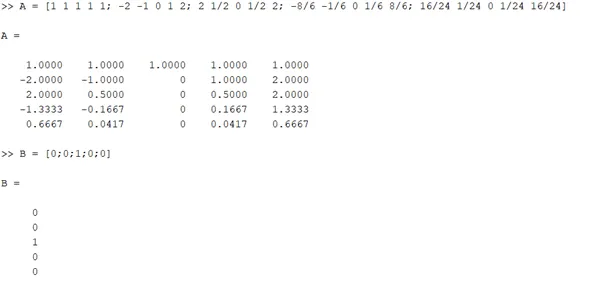
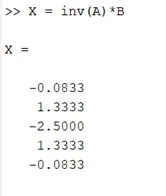
Finally the equation reduces to

`(del^2u)/(delx^2) = (a*f_(i-2) + b* f_(i-1) + c* f_(i) + d* f_(i+1) + e* f_(i+2))/(Deltax^2)`

Substituting the values of a,b,c,d & e in the above equation we get

`(del^2u)/(delx^2) = (-0.0833*f_(i-2) + 1.333* f_(i-1) – 2.5* f_(i) + 1.3333* f_(i+1) – 0.0833* f_(i+2))/(Deltax^2)`

Skewed right-sided difference

The number of nodes = p+q

Number of nodes = 6

Similarly for skewed right hand side we can write the table as

	f(x)	`Deltax*f’(x)`	`Deltax^2*f”(x)`	`Deltax^3*f”’(x)`	`Deltax^4* f_i^('v)`	`Deltax^5* f_i^(v)`
`f_(i)`	a	0	0	0	0	0
`f_(i+1)`	b	b	`b/2`	`b/6`	`b/24`	`b/120`
`f_(i+2)`	c	`2*c`	`4/2*c`	`8/6*c`	`16/24*c`	`32/120*c`
`f_(i+3)`	d	`3*d`	`9/2*d`	`27/6*d`	`81/24*d`	`243/120*d`
`f_(i+4)`	e	`4*e`	`16/2*e`	`64/6*e`	`256/24*e`	`1024/120*e`
`f_(i+5)`	g	`5*g`	`25/2*g`	`125/6*g`	`625/24*g`	`3125/120*g`
	0	0	1	0	0	0

`A = [[1,1,1,1,1,1],[0,1,2,3,4,5],[0,1/2,4/2,9/2,16/2,25/2],[0,1/6,8/6,27/6,64/6,125/6],[0,1/24,16/24,81/24,256/24,625/24],[0,1/120,32/120,243/120,1024/120,3125/120]]`

`B = [[0],[0],[1],[0],[0],[0]]`

Therefore, AX = B

Calculating in matlab we get

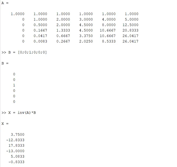
Finally the equation reduces to

`(del^2u)/(delx^2) = (a*f_(i) + b* f_(i+1) + c* f_(i+2) + d* f_(i+3) + e* f_(i+4) + g*f_(i+5))/(Deltax^2)`

Substituting the values of a,b,c,d,e & g in the above equation we get

`(del^2u)/(delx^2) = (3.75*f_(i) – 12.8333* f_(i+1) + 17.8333* f_(i+2) - 13* f_(i+3) + 5.0833* f_(i+4) – 0.8333*f_(i+5))/(Deltax^2)`

Skewed left-sided difference

Number of nodes = p+q

Number of nodes = 6

Similarly for skewed right hand side we can write the table as

	f(x)	`Deltax*f’(x)`	`Deltax^2*f”(x)`	`Deltax^3*f”’(x)`	`Deltax^4* f_i^('v)`	`Deltax^5* f_i^(v)`
`f_(i)`	a	0	0	0	0	0
`f_(i-1)`	b	-b	`b/2`	`-b/6`	`b/24`	`-b/120`
`f_(i-2)`	c	`-2*c`	`4/2*c`	`-8/6*c`	`16/24*c`	`-32/120*c`
`f_(i-3)`	d	`-3*d`	`9/2*d`	`-27/6*d`	`81/24*d`	`-243/120*d`
`f_(i-4)`	e	`-4*e`	`16/2*e`	`-64/6*e`	`256/24*e`	`-1024/120*e`
`f_(i-5)`	g	`-5*g`	`25/2*g`	`-125/6*g`	`625/24*g`	`-3125/120*g`
	0	0	1	0	0	0

`A = [[1,1,1,1,1,1],[0,-1,-2,-3,-4,-5],[0,1/2,4/2,9/2,16/2,25/2],[0,-1/6,-8/6,-27/6,-64/6,-125/6],[0,1/24,16/24,81/24,256/24,625/24],[0,-1/120,-32/120,-243/120,-1024/120,-3125/120]]`

`B = [[0],[0],[1],[0],[0],[0]]`

Therefore, AX = B

Calculating in matlab we get

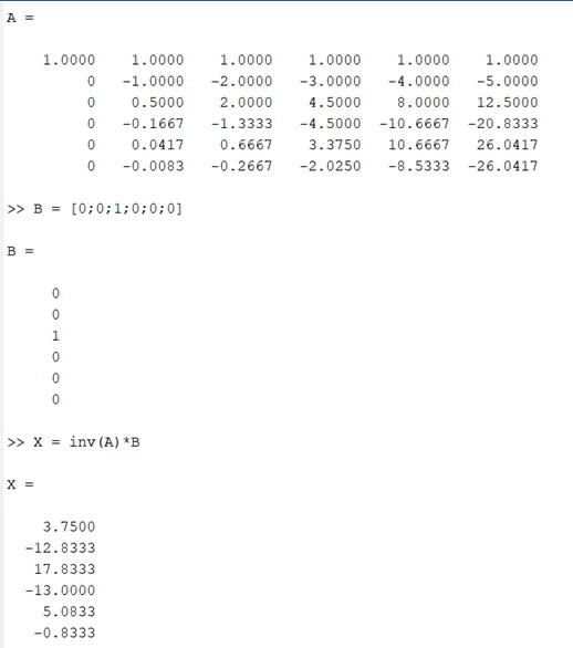
Finally the equation reduces to

`(del^2u)/(delx^2) = (a*f_(i) + b* f_(i-1) + c* f_(i-2) + d* f_(i-3) + e* f_(i-4) + g*f_(i-5))/(Deltax^2)`

Substituting the values of a,b,c,d,e & g in the above equation we get

`(del^2u)/(delx^2) = (3.75*f_(i) – 12.8333* f_(i-1) + 17.8333* f_(i-2) - 13* f_(i-3) + 5.0833* f_(i-4) – 0.8333*f_(i-5))/(Deltax^2)`

Matlab Program for calculating the error

x=pi/3;
dx=linspace(pi/40,pi/4000,4000);
%analytical solution
F = exp(x)*cos(x);
%Second derivative 
analytical_solution = -2*exp(x)*sin(x);

for i = 1:length(dx)
[central_approximation(i),right_sided_approximation(i),left_sided_approximation(i)] = error(x,dx(i));
central_error(i) = abs(central_approximation(i)-analytical_solution);
right_sided_error(i) = abs(right_sided_approximation(i)-analytical_solution);
left_sided_error(i) = abs(left_sided_approximation(i)-analytical_solution);
end

loglog(dx,central_error)
hold on
loglog(dx,right_sided_error)
loglog(dx,left_sided_error)
xlabel('dx')
ylabel('errors')
legend('central error', 'right sided error' , 'left sided error')

Matlab Function

function [central_differencing,right_sided_differencing,left_sided_differencing] = error(x,dx)
%Calculating Numerical approximation
central_differencing = (((-0.0833)*(exp(x-(2*dx)))*(cos(x-(2*dx)))) + ((1.3333)*(exp(x-dx))*(cos(x-dx))) - ((2.5)*(exp(x))*(cos(x))) + ((1.3333)*(exp(x+dx))*(cos(x+dx))) - ((0.0833)*(exp(x+(2*dx)))*(cos(x+(2*dx)))))/(dx^2);
right_sided_differencing = (((3.75)*(exp(x))*(cos(x))) - ((12.8333)*(exp(x+dx))*(cos(x+dx))) + ((17.8333)*(exp(x+(2*dx)))*(cos(x+(2*dx)))) - ((13)*(exp(x+(3*dx)))*(cos(x+(3*dx)))) + ((5.0833)*(exp(x+(4*dx)))*(cos(x+(4*dx)))) - ((0.8333)*(exp(x+(5*dx)))*(cos(x+(5*dx)))))/(dx^2);
left_sided_differencing = (((3.75)*(exp(x))*(cos(x))) - ((12.8333)*(exp(x-dx))*(cos(x-dx))) + ((17.8333)*exp((x-(2*dx)))*(cos(x-(2*dx)))) - ((13)*(exp(x-(3*dx)))*(cos(x-(3*dx)))) + ((5.0833)*(exp(x-(4*dx)))*(cos(x-(4*dx)))) - ((0.8333)*(exp(x-(5*dx)))*(cos(x-(5*dx)))))/(dx^2);
end

Results

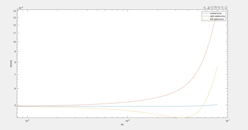
Conclusion:- From the above graph we can see that the error we get from the central differencing method is low as compared to the other two methods

Why a skewed scheme is useful?

If in a system, there is no sufficient information along both the sides of point of interest, then there we cannot use Central Differencing method. So in that case a skewed scheme is useful

What can a skewed scheme do that a CD scheme cannot?

We cannot apply Central Differencing scheme at boundary nodes due to unavailability of information on right and left side of the node. So there we apply a skewed scheme