Week 3.3 - Air standard Cycle

Aim: To write a code that can solve an otto cycle and make plots for it.

Objective:

• The code should create a PV diagram.
• Finding the thermal efficiency of the engine.

Introduction:

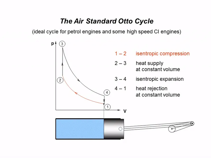
• The system that is performing an ideal Otto cycle goes through a series of four internally reversible processes: two isentropic (reversible adiabatic) processes alternated with two isochoric processes.

1. Isentropic compression (compression stroke): Gas (fuel-air mixture) is compressed adiabatically from state 1 to state 2 as the piston moves from bottom dead center to top dead center during an isentropic compression (compression stroke). The environment exerts some influence over the gas by raising its internal energy (temperature) and compressing it. Entropy, on the other hand, doesn't change. The compression ratio refers to the volume changes and their ratio (V1 / V2).
2. Isochoric compression (ignition phase): During this phase (between states 2 and 3), a constant-volume heat transfer from an outside source occurs to the air while the piston is at top dead center rest. This procedure is meant to simulate the rapid burning that occurs after the fuel-air mixture is ignited and injected into the combustion chamber. The ratio (P3 / P2) is referred to as the "explosion ratio" as the pressure increases.
3. Isentropic expansion (power stroke): As the piston moves from top dead center to bottom dead center, the gas expands adiabatically from state 3 to state 4. The gas exerts a force on the piston and loses internal energy equal to the force it exerts on the environment. The gas exerts a force on the surrounding area (the piston) and expends internal energy in proportion to the work it does. The entropy is unchanged once more. In the Otto cycle, the volume ratio (V4 / V3), also known as the isentropic expansion ratio, is equal to the compression ratio.
4. Isochoric decompression (Exhaust stroke): also known as isochoric decompression Heat is removed from the air during this phase of the cycle, which is completed by a constant-volume process with the piston at the bottom dead center. From point 4 to point 1, the working gas pressure immediately decreases. Point 4 is where the exhaust valve opens. After this decompression comes to the exhaust stroke. The gaseous mixture is vented to the atmosphere as the piston moves from the bottom dead center (point 1) to the top dead center (point 0), with the exhaust valve open, and the process is restarted.

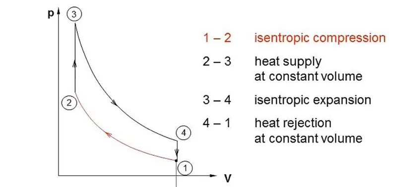
Following is a description of the processes:

• Process 1-2: As the piston moves from the bottom dead center (BDC) to the top dead center, the working fluid is compressed isentropically (TDC).
• Process 2-3: In this case, the SI causes a quick burning to happen inside the piston; as a result, the heat addition happens at a constant volume.
• Process 3-4: During this step, the working fluid expands isentropically to create the cycle's useful work.
• Process 4-1: constant volume thermal removal. In real-world settings, the heat is dispersed by releasing exhaust gas into the atmosphere.

FACTORS ENTAILED:

• Compression ratio (cr): It is the ratio of volume before compression to the volume after compression.Compression ratio (cr) = Volume before compression/volume after compression also, Compression ratio (cr) = VS+VcVcVS+VcVc

Where,

V1 = Volume before compression = V_Swept+V_clearance

V2 = Volume after Compression = V_Clearance

Vs = V_swept

Vc = V_clearance

Hence, Compression ratio (Cr) = V1V2V1V2

• Expansion ratio (Er): It is the ratio of volume after Expansion to the volume before compression.

• Note: (Cr=Er) where for the otto cycle compression ratio = expansion ratio.
• Expansion ratio (Er): V4V3V4V3

• Swept Volume and Clearance Volume: Swept Volume (V_s) is a volume Before compression stroke. Also known as stoke volume and Displacement volume. Similarly, Clearance volume (V_c) is the volume after compression stroke.

Input parameters:

• Initial pressure & Temperature: P1= 80kpa, T1=400K
• Engine Geometry parameters: Bore (D) = 0.3m, Stroke (L)=0.8m, Connecting rod (con_rod)= 0.10m and Compression ratio (Cr) = 8

Considered Parameters:

• Clearance volume Vc=Vscr−1Vc=Vscr-1
• Swept volume: Vs=(π4)⋅D2⋅LVs=(π4)⋅D2⋅L
• Pressure at P2: P2=P1⋅(cr)γP2=P1⋅(cr)γ
• Temperature at T2: T2=P2⋅V2⋅T1P1⋅V1T2=P2⋅V2⋅T1P1⋅V1
• Volume at P2: V3=V2V3=V2
• Pressure at P3: P3=P2⋅T3T2P3=P2⋅T3T2
• Volume at P4: V1=V4V1=V4
• Pressure at P4; P4=P3⋅(V3V4)γP4=P3⋅(V3V4)γ

Matlab Program:

• Initial Program:

%Inputs

gamma=1.4
t3=2778

%State Variable P1 in Kpa and t1 in K

P1=80
t1=400

%engine Geometry parameter

bore = 0.03
stroke = 0.18
con_rod= 0.10
cr= 10

%Swept volume and clearance volume

v_swept = (pi/4)*bore^2*stroke;
v_clearance = v_swept/(cr-1);
v1=v_swept+v_clearance
v2=v_clearance

%state variable at point 2
%p1v1^gamma=p2v2^gamma
%p2=p1*(v1/v2)^gamma=p1*cr^gamma
p2=p1*cr^gamma;

%p1v1/t1=p2v2/t2| t2= p2*v2*t1/(P1*v1)
t2=p2*v2*t1/(p1*v1);

%state variable at point 3
v3=v2

%p3vp/t3=p2v2/t2| p3= p2*t3/t2
p3= p2*t3/t2

%state variable at state point 4
v4=v1
p4 = p3*(v3/v4)^gamma;

%p3v3^gamma=p4v4^gamma| p4=p3(v3/v4)^gamma
p4=p3*(v3/v4)^gamma

%thermal efficiency
Percentage_Efficiency = (1-(cr^(gamma-1))^-1)*100

%plotting
figure(1)
hold on
plot(v1,p1,'*','color','r')
plot(v2,p2,'*','color','r')
plot(v3,p3,'*','color','r')
plot(v4,p4,'*','color','r')
xlabel('Volume(m^3)')
ylabel ('pressure (KPa)')

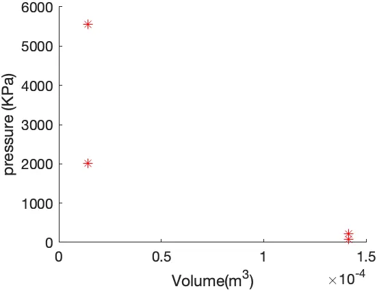
We cannot join them from the line because isentropic processes do not have a constant slope. If we try, we get the result as follows by using the following command, which is an Error.

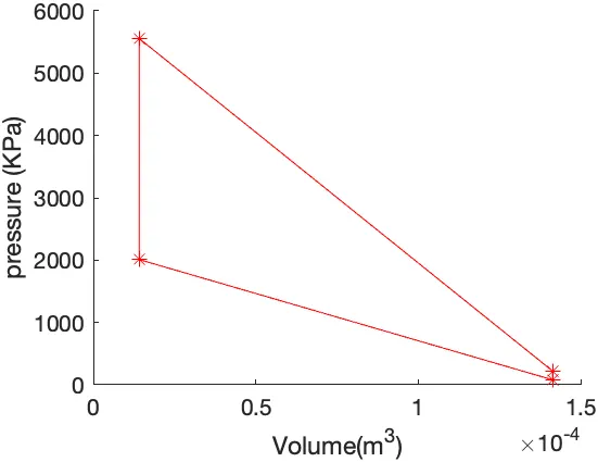
Error Elimination:

• For the right plot, using a function command to execute in the initial Matlab program, results in the perfect plotting according to the formulae considered in three terms, and altogether the PV diagram plots exactly to the program.

function [V] = engine_kinematics(bore,stroke,con_rod,cr,start_crank,end_crank)
 
 a=stroke/2;
 R=con_rod/a;
 V_s=(pi/4) * bore^2 * stroke;
 V_c = V_s/(cr-1);
 
 angle = linspace(start_crank,end_crank,100);
 
 %formula
 term1 = 0.5*(cr-1);
 term2= R+1-cosd(angle);
 term3=(R^2-sind(angle).^2).^0.5;
 
 V=(1+term1*(term2-term3)).*V_c;
 end

• We are using the same parameters as before in this case, but a different formula is required to calculate the volume change within the combustion chamber. The formula below can be used to determine the necessary relationship.

• V/Vc = 1+ 0.5(cr-10)* [ R+1 -cos(angle) - (R^2 -sin^2(angle)^0.5]

• The above formula is divided into three subformulas as follows
• term1 = 0.5⋅(cr−1);0.5⋅(cr-1);
• term2 = R+1−cosd(θ);R+1-cosd(θ);
• term3 = (R2−sind2(θ))0.5;(R2-sind2(θ))0.5;

The final set of formulas:

V=(1+term⋅(term2−term3))⋅VcV=(1+term⋅(term2-term3))⋅Vc

Where,

R= length of connecting rod/ crankpin radius.

• Using the above program in the first set of programs for getting the PV diagram correctly.
• Uthe following command, Function [V] =piston_kinematics(bore,stroke,con_rod,cr,start_crank,end_crank) able to correct the error in the first program.
• we are using this function for the Pressure and volume changes in the compression and Expansion stroke, for the volume we can define the function as follows.

  v_expansion = piston_kinematics(bore,stroke,con_rod,cr,180,360);

• Where we know that p*v^gamma=constant.
• similarly, constant_c = p3*v3^gamma;
• v_expansion = piston_kinematics(bore,stroke,con_rod,cr,180,360);
• p_expansion = constant_c./v_expansion.^gamma;

Calculating Thermal Efficiency:

• Percentage_Efficiency = (1-(cr^(gamma-1))^-1)*100;

Final Matlab Program:

%Inputs

gamma=1.4
t3=2778

%State Variable p1 in kpa and t1 in K

p1=80
t1=400

%engine geometry parameter

bore = 0.03
stroke = 0.18
con_rod= 0.10
cr= 10

%Swept volume and clearance volume

v_swept = (pi/4)*bore^2*stroke;
v_clearance = v_swept/(cr-1);
v1=v_swept+v_clearance
v2=v_clearance

%state variable at point 2
%p1v1^gamma=p2v2^gamma
p2=P1*cr^gamma;
constant_c=P1*v1^gamma;

v_compression=engine_kinematics(bore,stroke,con_rod,cr,180,0);
p_compression=constant_c./v_compression.^gamma;
t2=p2*v2*t1/(P1*v1);

%state variable at point 3
v3=v2
p3= p2*t3/t2
constant_c=p3*v3^gamma;
v_expansion=engine_kinematics(bore,stroke,con_rod,cr,180,360);
p_expansion=constant_c./v_compression.^gamma;

%state variable at state point 4
v4=v1
p4=p3*(v3/v4)^gamma

%thermal efficiency
Percentage_Efficiency = (1-(cr^(gamma-1))^-1)*100

%plotting
figure(1)
hold on
plot(v_compression,p_compression,'linewidth',1.5,'color','c')
plot(v_expansion,p_expansion,'linewidth',1.5,'color','c')
plot([v2 v3],[p2 p3],'linewidth',1.5,'color','g')
plot([v4 v1],[p4 P1],'linewidth',1.5,'color','g')
plot(v1,P1,'*','color','r')
plot(v2,p2,'*','color','r')
plot(v3,p3,'*','color','r')
plot(v4,p4,'*','color','r')
xlabel('Volume(m^3)')
ylabel('pressure (KPa)')


plot([v1 v2 v3 v4],[P1 p2 p3 p4],'color','r')

Output:

• By executing the above final program in Matlab, we get,

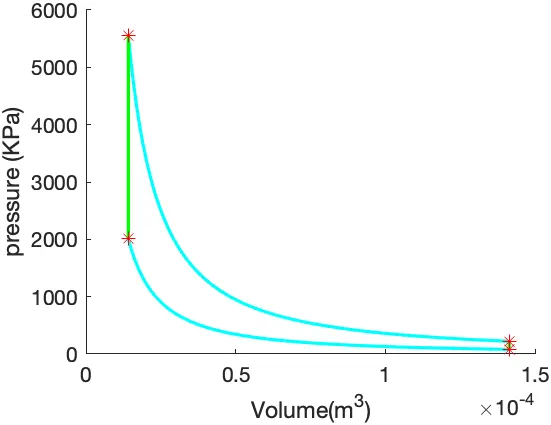
• Otto cycle plot of PV diagram.
• Thermal efficiency in percentage,

Conclusion:

• Otto cycle plot of PV diagram And the thermal efficiency in percentage is achieved using Matlab.

Reference:

• https://www.sciencedirect.com/topics/engineering/otto-cycle
• https://www.dailymotion.com/video/x41p8t0.