Week 2 Railwheel and Track

Simulation on Rail wheel and track:

Aim:-

To simulate the railwheel and track for their lifecycle, equivalent stress and strain, total deformation provided by the wheel running on the track by the given forces.

Objective:-

The main focus of this component is to evaluate the result of the product life cycle and the stress, strain, and total deformation in the static structural material. This component to be examined by two cases-

Case 1: Load of 100000 N.

Case 2: Load of 5 times of 100000 N.

Lastly implement user-defined results and compare both results in all aspects of the evaluation.

Introduction:

Rail wheel and track concept:

The train wheel or a rail wheel is specially designed for use of railway tracks. This rolling component(wheel) is especially pushed onto on axle and mounted directly on a railway carriage or locomotive or indirectly we can say a boogie. This wheel is cast or forged and is heated or treated to have a specific hardness. New wheels are trued, using a lathe, to a specific profile before being pressed onto an axle. All wheel profile must be regularly checked to ensure proper interaction between the rail and wheel. Incorrectly trued or worn out wheels can increase rolling resistance, reduce energy efficiency and many even cause a derailment.

Wheel Geometry and Flange, most train wheels have a conical geometry, which is the initial means of keeping the train motion aligned with the track. The train wheels have a flange on one side to keep the wheels and hence the train, running on the rails when the limits of geometry based alignments are reached.

Procedure:

I. Geometry-

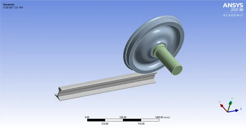
The CAD model of Rail wheel and track is imported in ANSYS static structural environment. It comprises of three major components namely running grail, wheel and shaft.

II. Material-

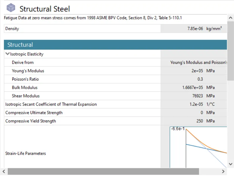
We have performed the analysis using 'Structural steel' as the material for the analysis of Rail wheel and track.

The Detailed engineering data of material is as shown in the below image-

III. Connection Details-

(a) Contact Details:

1. Frictional Contact-

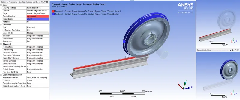
Frictional contact is given between faces of running grail and wheel as seen in the image below. As, these contact is selected through 'Frictional' contact with a frictional coefficient of 0.3. In this type, the formulation is taken as 'Program Controlled' and Interference treatment is selected by default.

2. Frictionless Contact-

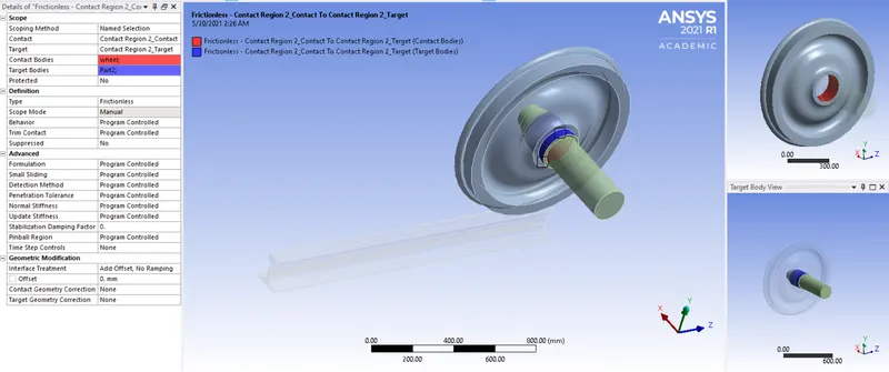
Frictionaless contact is given between faces of wheel and shaft as seen in the image below. As, these contact is selected through 'Frictionaless' contact. In this type, the formulation is taken as 'Program Controlled' and Interference treatment is selected by default.

(b) Joint Details:

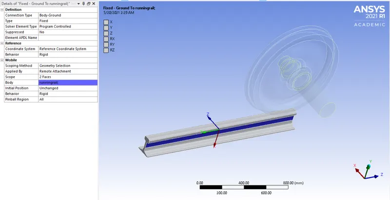
1. Fixed- Ground to running grail:

As, running grail has given fixed joint with connection type as 'Body-Ground' and then we have to fix as joint as fixed type. After that we have to select the geometry as running grail. Then, it can be shown in below figure.

2. Translational- Ground to Part 2:

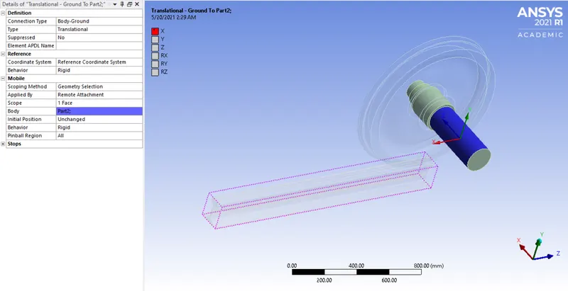
As, part 2. will be given as translational joint so that it can move forward X direction. It has given translational joint with connection type as 'Body-Ground' and then we have to fix as joint as translational type. After that we have to select the geometry as Part 2. Then, it can be shown in below figure.

3. Planar- Ground to wheel:

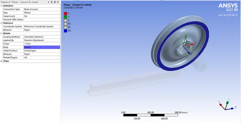
As, wheel will be given as planar joint with connection type as 'Body-Ground' and then we have to fix as joint as planar type. After that we have to select the geometry as wheel. Then, it can be shown in below figure.

IV. Mesh-

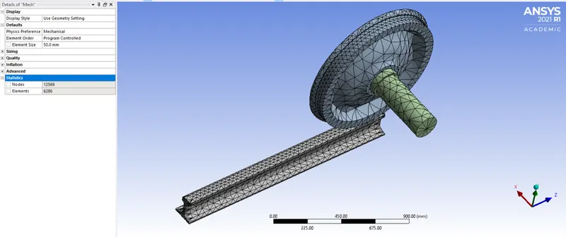
As, we have done mesh of 50 mm so that the fine mesh with 12569 nodes and 6286 elements and also we have done face sizing for mesh of 35 mm which is sufficient to carry out simulation giving desired results.

V. Boundary conditions and Analysis Settings-

(a) Analysis Settings-

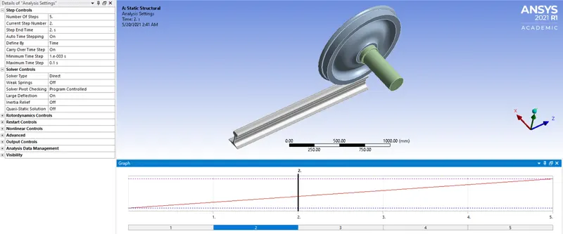
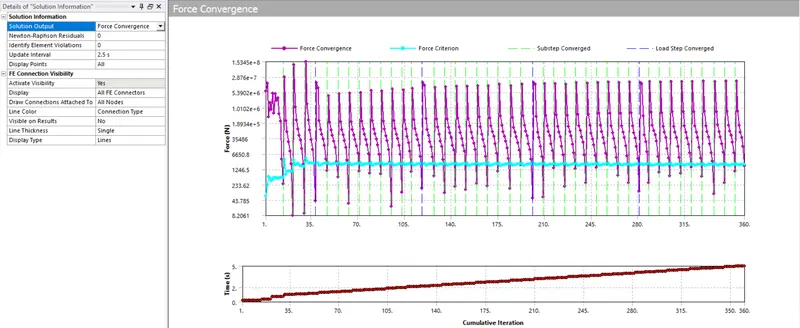
For this analysis total number of steps is set to '6'. Basically, for the first initial step, the Auto time stepping must be 'Program controlled.' Then, Large deflection must be 'On' so as to account for changes in stiffness due to change in shape of gears and primarily non-linear controls such as Force convergence should be 'On'. Also, the output controls parameters must be on. Then, remaining 5 steps, we should keep the Auto time stepping must be 'On'. Then, we have to define it by time and change the setting of Carry over time must be ON, and maximum and minimum time will be 0.1 and 0.001 sec.

(b) Joint load details-

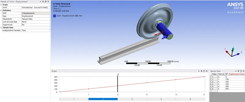
1. Joint-Displacement:

Basically, we have preferred joint as 'Translational-Ground to part 2.' Then, we have to set type as 'Displacement' and magnitude as 'Tabular' form. After that, we have to set displacement as 100 mm for the 6 steps.

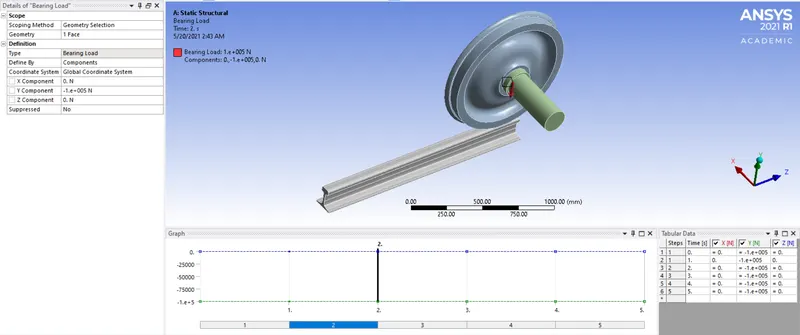
2. Bearing Load:(100 KN)

As, we have to select the geometry face, then we have to select the type as 'Bearing load', then we have to select define type as component and Y coordinate as -1e5 N for all basic steps.

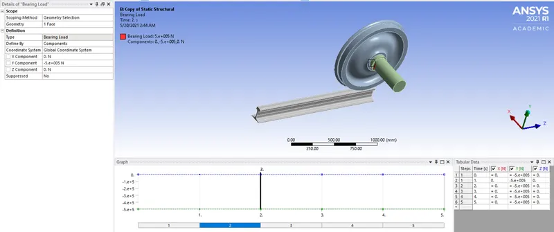
3. Bearing Load:(500 KN)

As, we have to select the geometry face, then we have to select the type as 'Bearing load', then we have to select define type as component and Y coordinate as -5e5 N for all basic steps.

VI. Post-processing and Results-

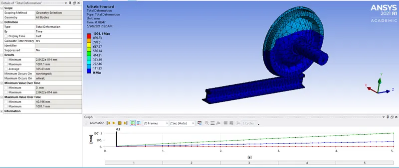
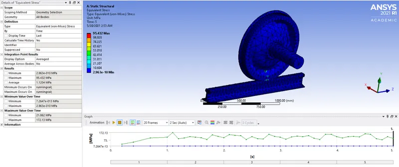
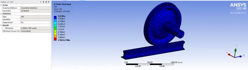
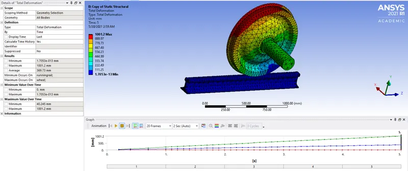
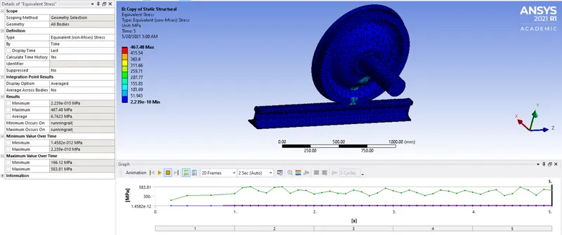
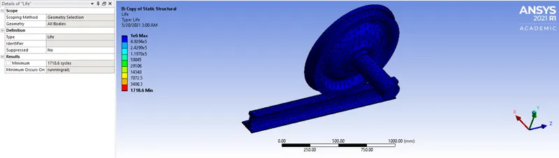
Now, we have to compare the bearing load of 100KN and 500KN. Then, we have to analyze the result for Total deformation, Equivalent stress, Equivalent strain and Life cycle. The results for each case as shown below-

Case 1- For 100 KN

I. Total deformation:

II. Equivalent stress:

III. Life cycle:

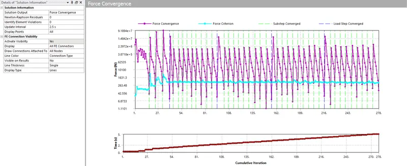
IV. Force convergence Graph:

Case 2- For 500 KN

I. Total deformation:

II. Equivalent stress:

III. Life cycle:

IV. Force convergence Graph:

Case 3: User Defined result

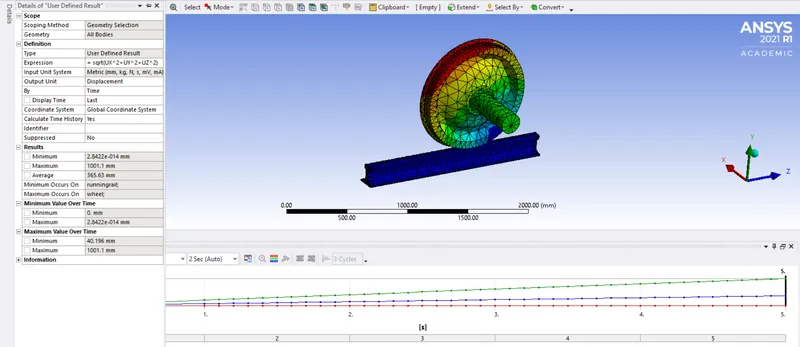
100 KN 500 KN

Post processing Results and Summary:

Sr. No	Statistical Analysis	100 KN	500 KN
1.	Maximum Equivalent stress	95.432 MPa	467.48 MPa
2.	Minimum Equivalent stress	2.963e-010 MPa	2.239e-010 MPa
3.	Maximum Total Deformation	100.1 mm	1001.2 mm
4.	Minimum Total Deformation	0	1.7053e-013
5.	Minimum Life cycle	5.56e+005 cycles	1718.6 cycles

Conclusion:

As, the result shows that the load increases, as the force on the trackwheel simulation increases, the equivalent stress and deformation increases i.e. the force is directly proportional to the stress value. And the life cycle for both loads is 1e^6 max.

After evaluating the user-defined result for both loads as we have take the result for both loads. Then the expression used to evaluate and the result expression used for total deformation is sqrt(UX^2+UY^2+UZ^2) and the output unit is displacement. By analyzing the result, the deformation in both cases is same.