Week 2 Railwheel and Track

Objective : To perform the simulation of motion of a rail wheel on a track and obtain the desired output.

Procedure :

Setting up the simulation :

Setting up the simulation :


To set up the simulation, first we need to import the required material card of structural steel. This material can be found in the general materials library.


Structural Steel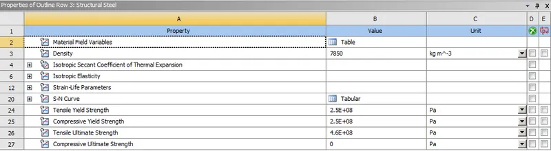





Importing geometry :
Next we import the geometry which theCAD file of the rail, wheel & shaft which has been provided. The parts are renamed as runningrail, wheel & shaft respectively for ease of understanding.

Material defintion :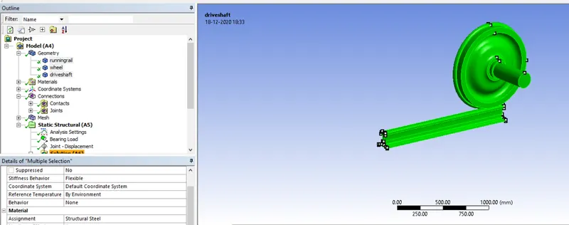

The material structural steel is assigned to all the components.

Then we will open Ansys mechanical to set up the rest of the simulation.
To set up the contact we go to connections-->contacts and open the contact card.
We will invert the contact and target bodies and rename the contact as definition based. We will create 2 contacts
1)Between Rail & wheel
2)Between shaft & wheel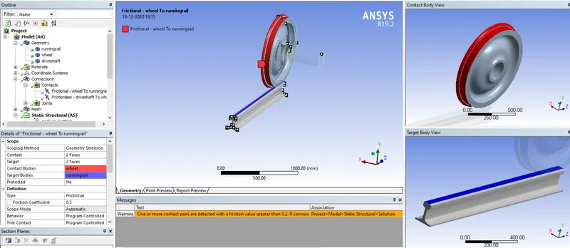

For the contact between rail & wheel select contact type as frictional,
Coefficient of friction = 0.3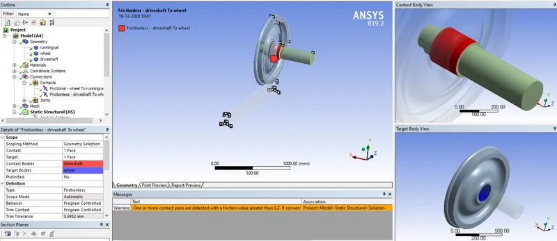


For the contact between wheel & shaft select contact type as frictionless as shown above. Thus contact definition is complete


Next we define the joints for the simulation.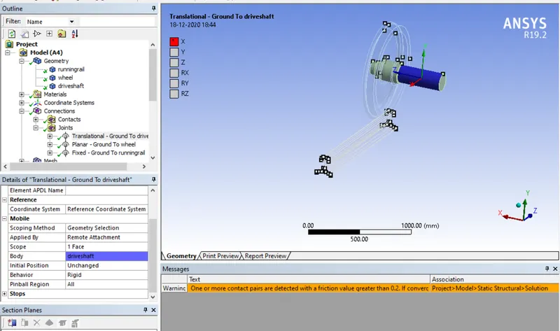


First we define the body-to-ground translational joint for the shaft. This is to enable it to move straight along the direction of motion of the wheel. Select the co-ordinate system geometry so that the direction of motion aligns with the x-axis as shown above.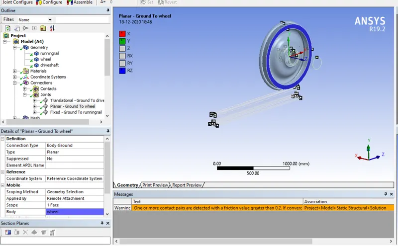


Next we define a body-to-ground planar joint to keep the wheel locked in lateral motion and enabling it to rotate about its own axis as the shaft moves forward. For the scope we select the back face of the wheel as shown above.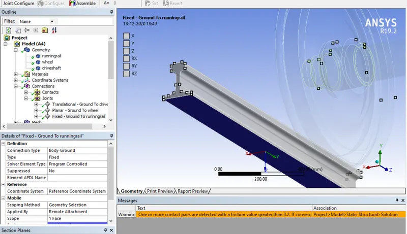


Finally we define a body-to-ground fixed type joint to constrain the rail to tthe ground to prevent its motion during the simulation. For the scope we select the lower face of the rail as shown above.


Next a general mesh is generated of 30 mm with face sizing applied of 10mm on the two areas in contact (i.e. rail surface and outer wheel circumference.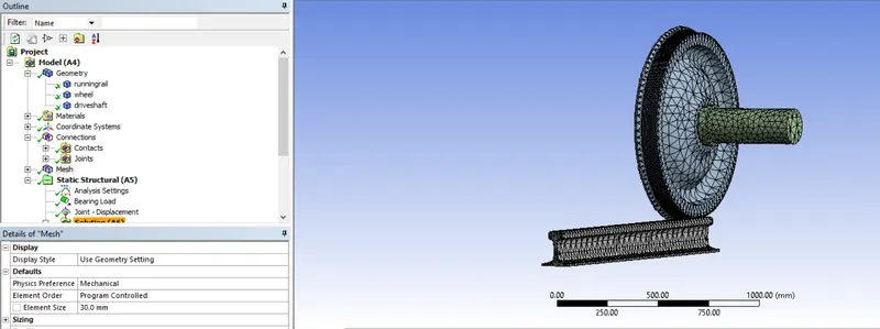

The face sizing is applied since that is the surface in contact and which will experience loads hence we want accurate results hence we apply a finer mesh in these regions. The selected areas for face sizing are shown below.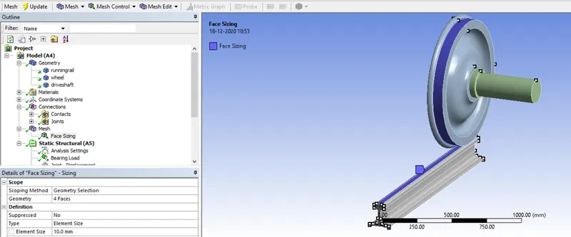



Creation of load conditions : Next we assign the translational motion to the wheel shaft. This is done by providing displacement in the form of 5 increments each of 100 mm each.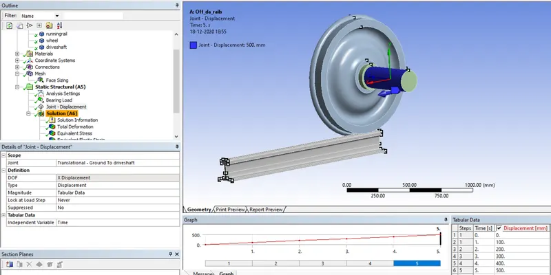


We verify that the direction of translational is in the one which we want along the length of the rail.

For the second load, we provide a bearing load on the inner race of the wheel to simulate the mass of the carriage which will be carried by the wheel.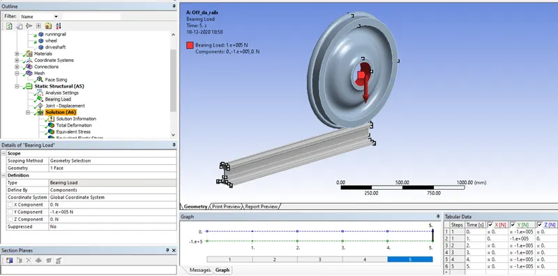

A load of 10,000N is applied in the downward direction is applied on the wheel as shown by the red highlighted area above.

Setting up the analysis settings : Next the analysis settings are selected as shown below, inputting the values of number of steps, initial time-step, maximum/minimum timestep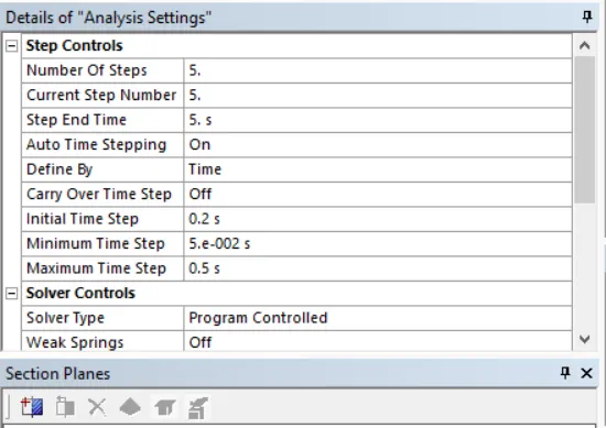

We select as total of 5 steps with the above given values for initial, maximum & minimum timestep.

Output Parameters : The following parameters are selected for output from the simulation.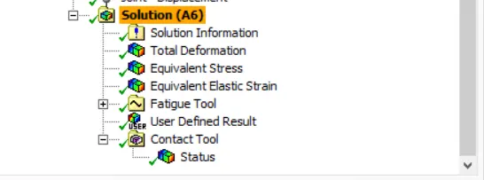

We have selected total deformation, equivalent stress, equivalent elastic strain along with a user defined result in which we will replicate the data obtained in total deformation output.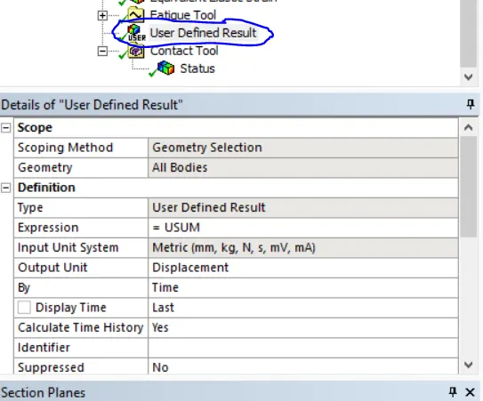

For user-defined result we input the correct expression USUM, give output unit as displacement as shown above.

Running the simulation :

Now we will run the simulation for the results.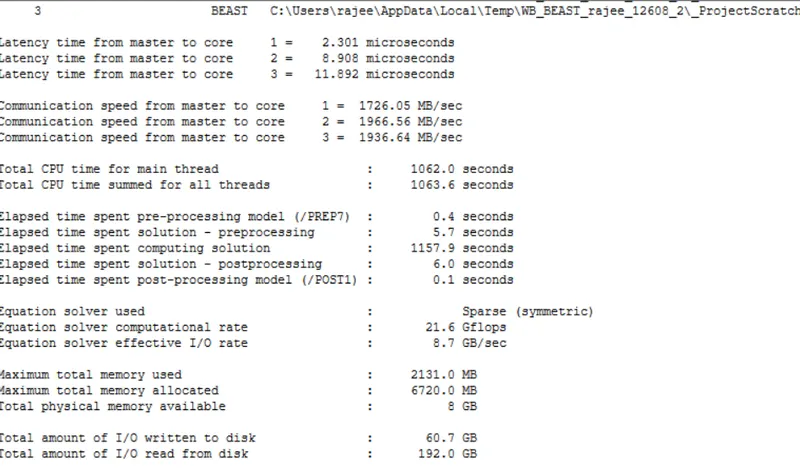

The simulation runs in about 20 minutes as shown above with a successful result.

During the run we can check whether the simulation is converging by checking the force convergence graph as shown below.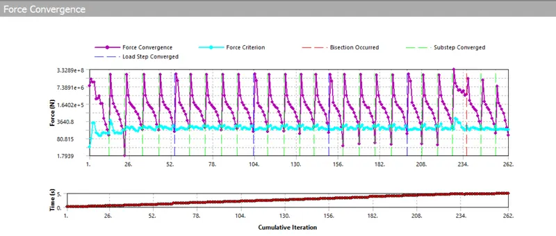

We will evalute the below results based on 2 loading conditions
1)Bearing load 100000 N
2)Bearing load 500000 N

Stress :
Case 1)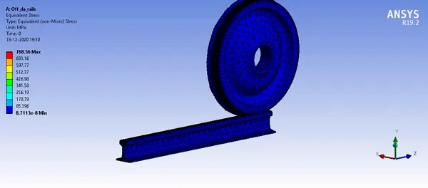

A peak stress of around 768 Mpa is obtained on the wheel toward the end of the run.

Case 2)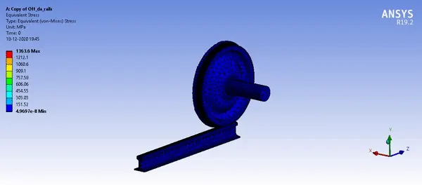

For the second load case a total stress of 1363.6 Mpa is generated on the wheel, which is a 77% increase in the stress from the previous load case.



Strain :
Case 1)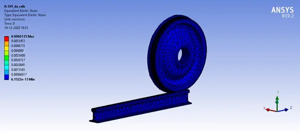

A peak strain of 0.6% is obtained on the wheel towards the end of the run as we can see above.

Case 2)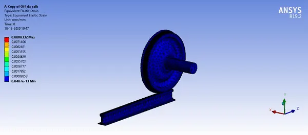

A peak strain of 0.8% in obtained on the wheel which is a 33% increase from the previous load case.

Total deformation :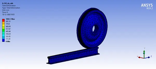

The total deformation as we can see above is 1002.7mm. This is an indication of the movement of the part as it is a simulation which includes moving parts.

Total deformation remains the same since we are providing the motion to the system which is independent of both the bearing load cases.

User defined results :
Now we will see the result of our user defined option.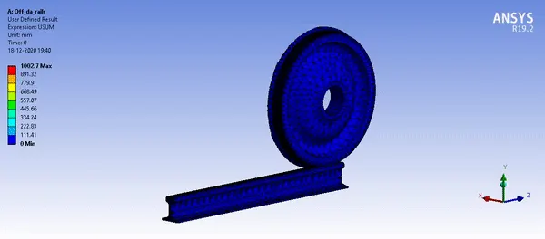

As we can see the result is exactly similar to toal deformation as shown above. Hence we have successfully executed a user defined output command.

Conclusion :
Hence the simulation of motion of wheel on a rail has been simulated and we have compared the results of different loading cases as well as generated the desired output from a user defined load case.

Result :
(Unable to attach file to portal directly,so attaching drive link)
Rail_sim is for standard load (case 1) , Rail_sim5 is for 5* bearing load (case 2)

Rail_sim