Week 2 - Flow over a Cylinder.

• FLOW OVER CYLINDER
• First of all we have go inside the Ansys workbench then we have click on Fluid Flow and drag on window.
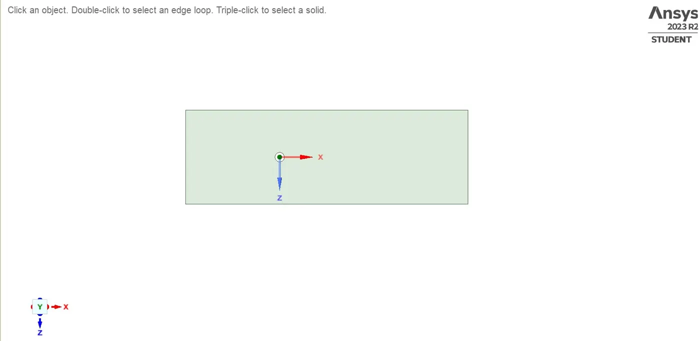
• We have to click on geometry inside Fluid Flow . We have click on File then select space claim option and change to meter inside units . we have to create a circle by given length 2m and we have take a construction line from circle mid point to left side by given length 20m and right side also we have take another construction line by given length 40m then create a construction line from left side end point to upward direction ,select the end point of z-axis point and create a rectangle by given length 20m and width is 60m.
• Once we completed geometry then we have click on Pull option and select geometry . By using Pull tool we converted to solid model. After we have to delete all construction line then close the geometry window.
• 
  
• We have to go inside the mesh option and generate the mesh . After meshing we got quadrilateral dominant shape inside mesh but we need triangular mesh for that we have to right click on mesh and select Insert , click on method option. Inside method we have to change to Triangle and select generate mesh then only we got triangular meshing.
• After meshing we saw inside circle that look like hexagon but we have to make it into circle . Again we have to right click on mesh ,select insert and click on sizing option . Inside sizing, we have select the circle boundary and apply in geometry . we have to change to no. of division inside the type and give the no. of division is 36. we have generate the mesh then only it look like circle.
• . Again we have to right click on mesh ,select insert and click on inflation . Inside this we have to select the full geometry and select the circle boundary then click on apply . we have to change to First layer thickness inside inflation option and we have to put the First layer height is 5e-3 . We have to give the maximum layer count is 6 then generate the mesh. We will got 6 layers inside the geometry. we have give the element size is 0.25 inside meshing and generate mesh .
• 
  
• 
  

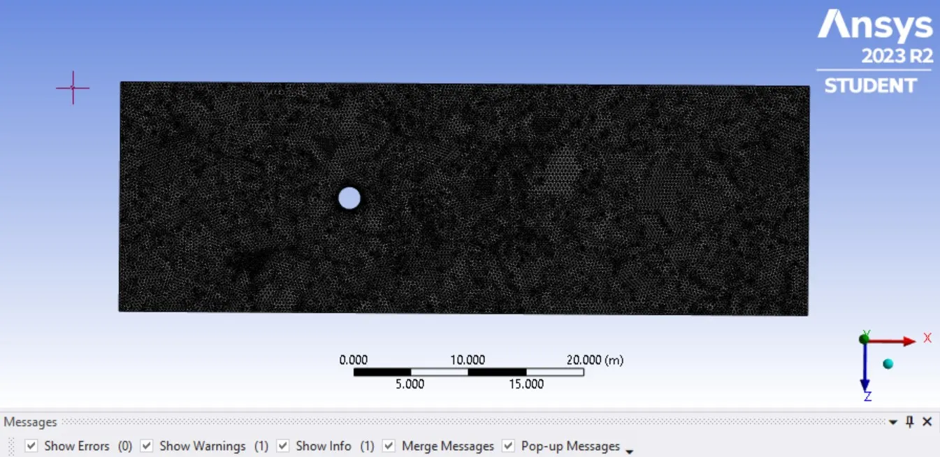
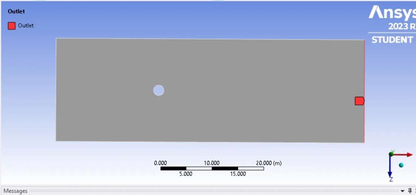
• Then we have to crate a named selection inside the model which are Inlet, Outlet, Wall and Symmetry.
• 
  
• 
  
• 
  
• 
  
• 
  
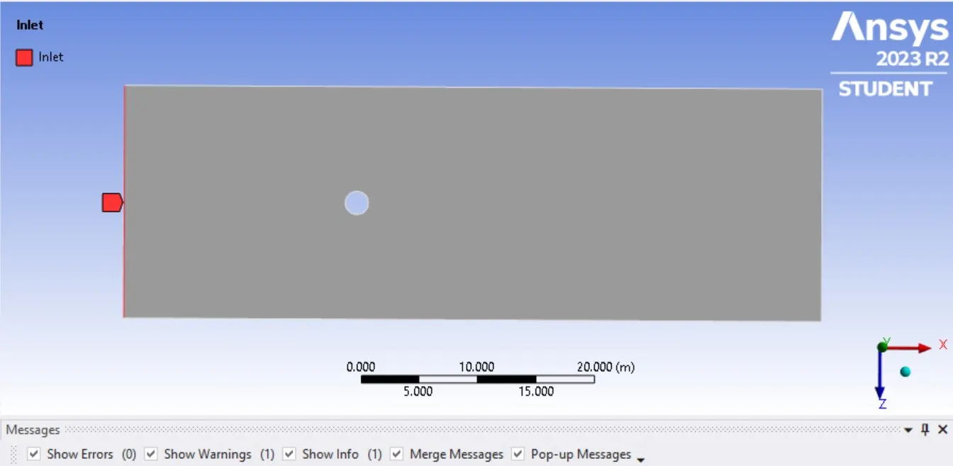
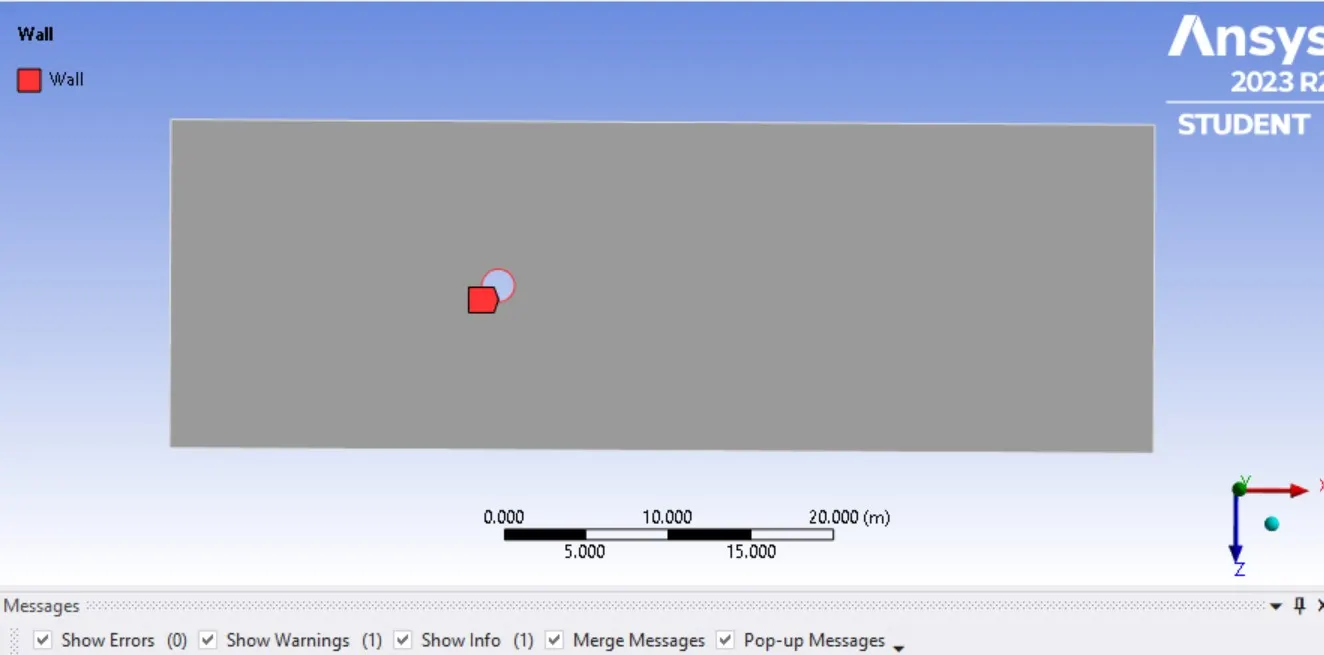
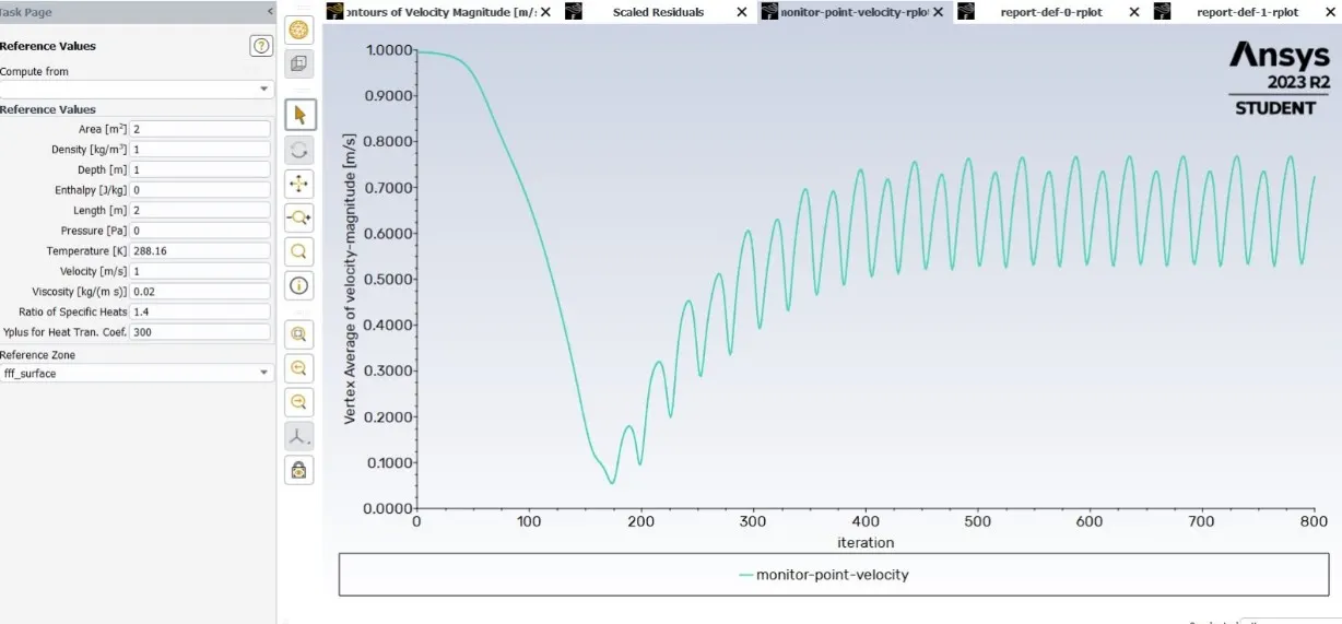
• We have to go inside setup .Then we have to check mesh by clicking perform check mesh after it showing ,your mesh is done... inside console if it is error showing inside the console then we have check meshing in the mesh. We have to select the Viscous option and click on laminar . Then we have to go inside the material option , inside material we have to select the fluent database option then we have to give the material type inside the fluid fluent material after that we have to copy and give the name like user-material .Then we have two material inside fluid fluent materials which one is air and another one is user-material , we need to delete air material but we cannot able delete one material. Then we have to go inside the Cell zone and change to User-material inside material name. After that we have return back to material option then delete the air material and change to User-material. we have to give the density value is 1 and viscosity is 0.02 ( we have change the value ,until we are getting good result inside plot).
• We have to go inside the Boundary condition and click on inlet then give the value of velocity is 1 m/s. we don't have to change the value inside the Wall , Outlet and symmetry.
• We have to go inside the result option, select create option then click on point and create a point which having x-axis is 10m and y-axis is 0 after that we have to give the name like monitor-point. We have select the definitions option ,Inside the definition we have to select the Vertex average then change to velocity in the field variable and also select monitor-point ,click on ok. After we have to go inside the Residual then remove thik mark in the monitor check convergence absolute criteria . We have to go inside the methods, In methods we have to change to Simple in the Scheme .
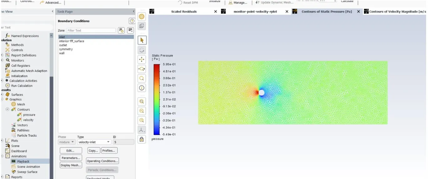
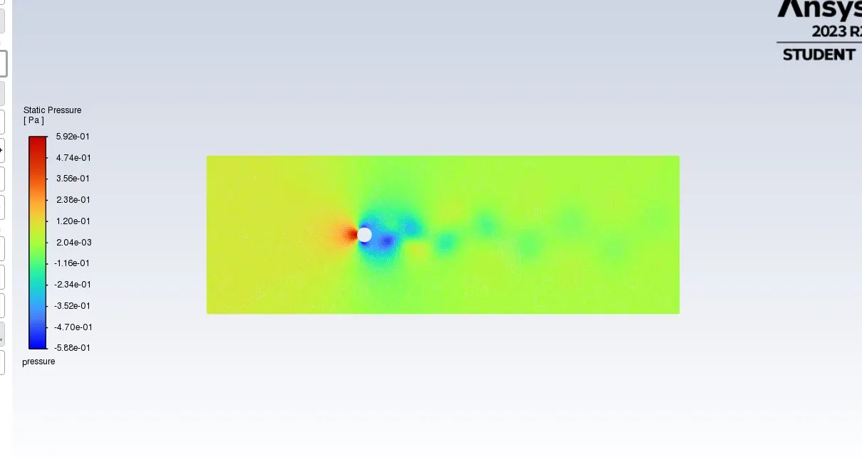
• We have to initialize the model by clicking the Initialization . Then we have to select contour and change to velocity in contour . Again create a another contour plot but we have to change to pressure in the contour. Both we created plots which one is Velocity and pressure. Then we got both plots inside the graphic.
• We have to select the Activities option then click on solution animations and the record after every is 10 number of time step.

STEADY STATE

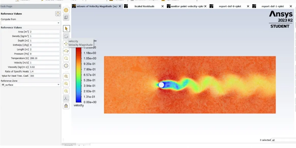
• We have select the General option and select the steady in the Time. Then go to solution >> click on Run calculation >> Give the no. of iteration is 500.
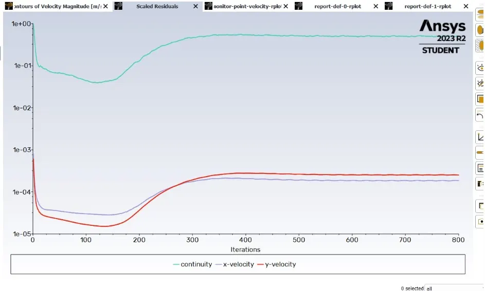
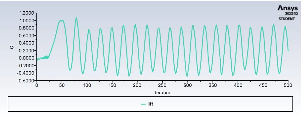
• Then the monitor point is going to be fluctuating with same ratio and we have to check the monitor point when its going to converge then we have to stop the iteration.
• 
  
• 
  
• 
  
• 
  
• Go to results >> click on Plots option >> click on FFT
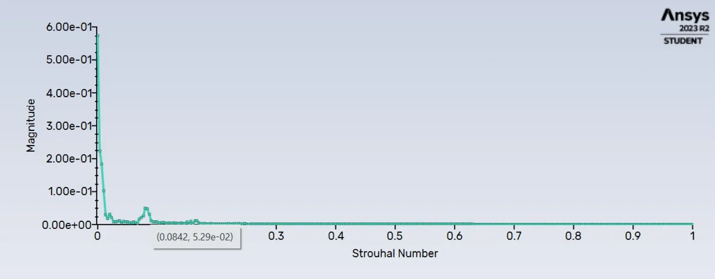
• Inside FFT we have to change to magnitude in Y-axis function and also we have to change to Strouhal number in X-axis function. We have to select the load input file then select the monitor point velocity and click on Plot FFT.
• We don't get good result in Strouhal number .
• 
  

UNSTEADY STATE

• We have select the General option and select the steady in the Time.
• We have to select the run calculation then we have give the value of time step size is 0.05 and number of time steps is 3000.
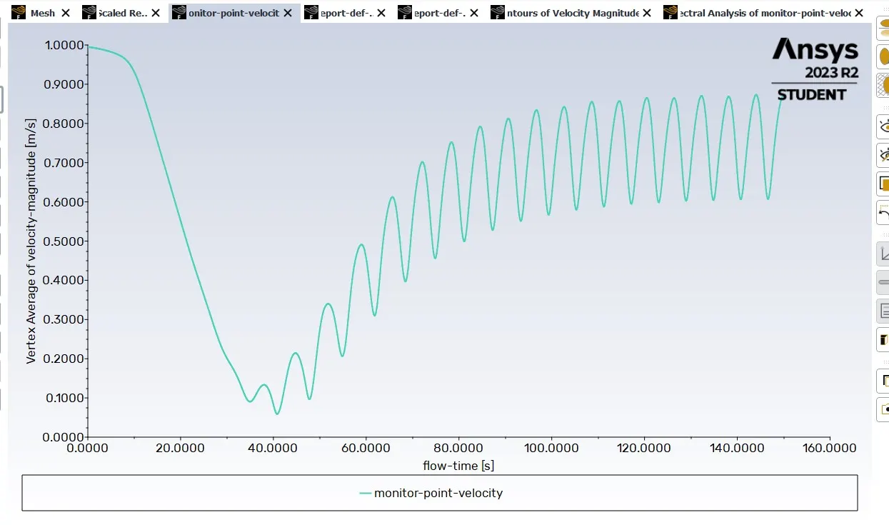
• If we run more then 3000 then the monitor point is going to be fluctuating with same ratio and we have to check the monitor point when its going to converge then we have to stop the iteration. It give us good result as compare to unsteady state.

• 
  
• 
  
• 
  
• 
  
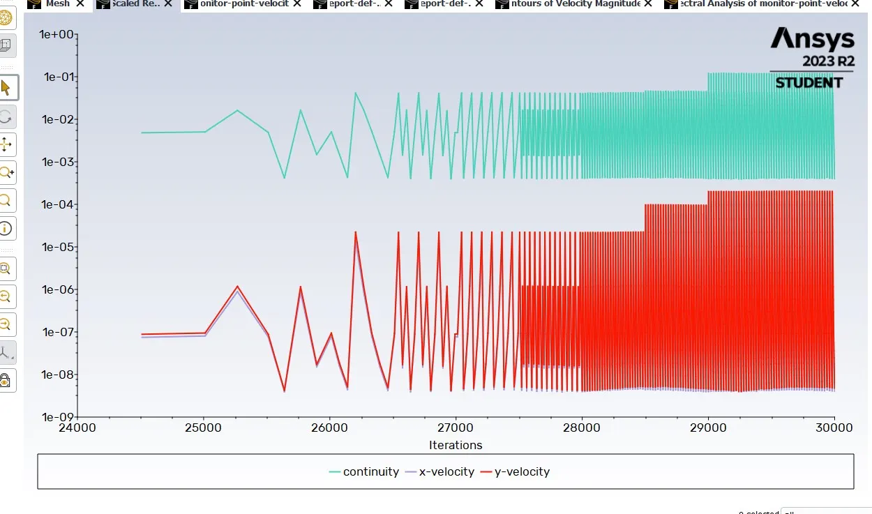
• Again Go to results >> click on Plots option >> click on FFT
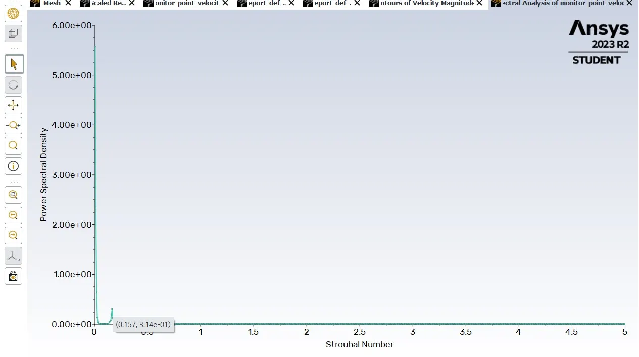
• Inside FFT we have to change to magnitude in Y-axis function and also we have to change to Strouhal number in X-axis function. We have to select the load input file then select the monitor point velocity and click on Plot FFT.
• We will got good result in Strouhal number after completed 3000 iteration.

• 
  

1. Discuss the effect of Reynolds number on the coefficient of drag :-

• We are going to Calculate the coefficient of drag and lift over a cylinder by setting the Reynolds number to 10,100,1000,10000 & 100000. (Run with steady solver)
• We have to go inside material and we have to give the Reynolds numbers which one is 0.2,0.02,0.002,0.0002 & 0.00002.
• We have to run the iteration for every Reynolds number then we will got output .
  
• We have to go inside definitions option then we have to click on Drag , In drag option we have to select the drag coefficient then we will got drag Coefficient report inside the graphic window and right click on report and click on compute then we will got output in the console,
• Again same procedure we have to follow then we will got lift coefficient report inside graphic window.
• If we run with Reynolds number is 10 then the drag coefficient value is 2.7136 and the lift coefficient is 0.0018 . In this Reynolds number , we didn't got good result .
• If we run with Reynolds number is 100 then the drag coefficient value is 1.3301 and the lift coefficient is -0.1048 . In this Reynolds number , we will got good result .
• If we run with Reynolds number is 1000 then the drag coefficient value is 1.2093 and the lift coefficient is 0.5090 . In this Reynolds number , we will got good result.
  
• If we run with Reynolds number is 10000 then the drag coefficient value is 1.3212 and the lift coefficient is 0.7731 . In this Reynolds number , we will got good result.
• If we run with Reynolds number is 100000 then the drag coefficient value is 1.3881 and the lift coefficient is 0.3237 . In this Reynolds number , we will got good result.

1. Expected results :-

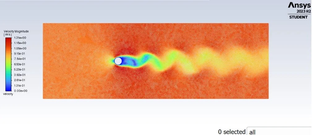
• First of all, we have to run with the Reynolds number is 100 . Then we have to give the iteration is 500 in steady state. After running the iteration then we have to wait and check the monitor point when its going to fluctuation and if the fluctuation is constantly happen that mean the monitor point is going to be converged .Then we have to stop the iteration. After we have check the vertex shedding is come behind cylinder or not. If the vertex shedding is not coming again we have to run continuously until we are getting vertex shedding inside the monitor point velocity plot .
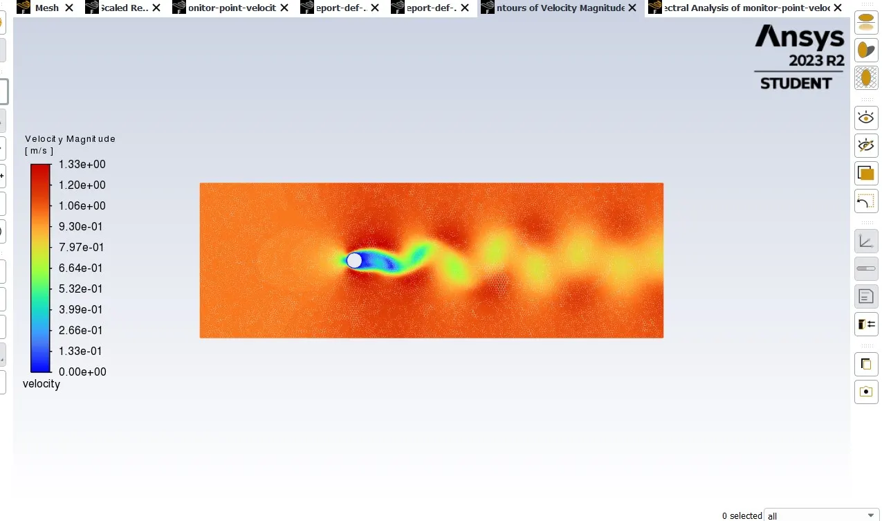
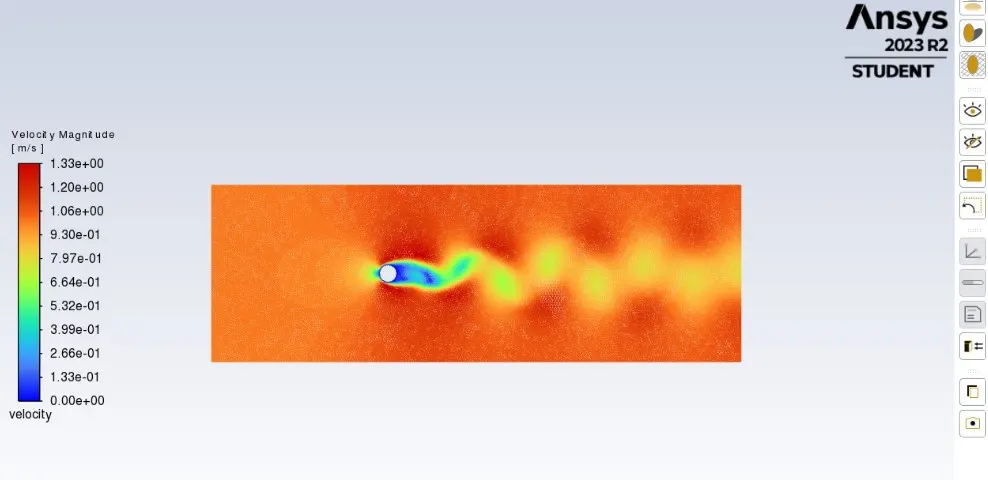
• Again we have to run more then 3000 because the monitor point is not going to fluctuate below 3000 in the unsteady state case. Then the monitor point is going to be fluctuating with same ratio and we have to check the monitor point when its going to converged then we have to stop the iteration and also we have to check the vertex shedding is coming or not behind cylinder .If the vertex shedding is coming we have to stop the iteration and if the vertex is not coming then we have to run until we are getting result.

1. Plots of the coefficient of drag :-

• If we run with Reynolds number is 10 then the drag coefficient then we will got plot like this.
• 
  
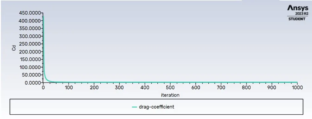
• If we run with Reynolds number is 100 then the drag coefficient then we will got plot like this.
• 
  
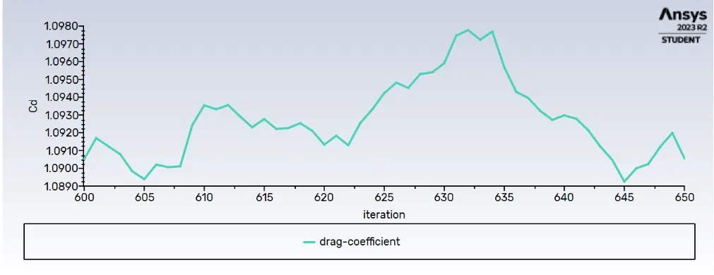
• If we run with Reynolds number is 1000 then the drag coefficient then we will got plot like this.
• 
  
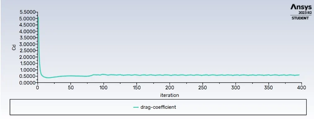
• If we run with Reynolds number is 10000 then the drag coefficient then we will got plot like this.
• 
  
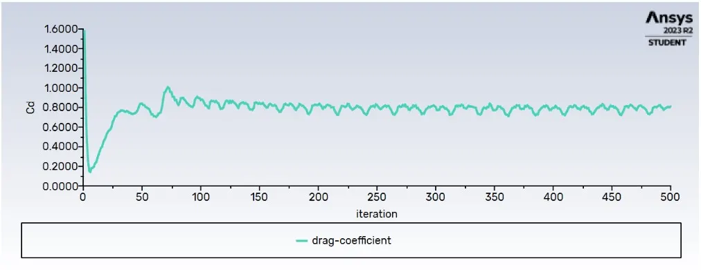
• If we run with Reynolds number is 100000 then the drag coefficient then we will got plot like this.
• 
  
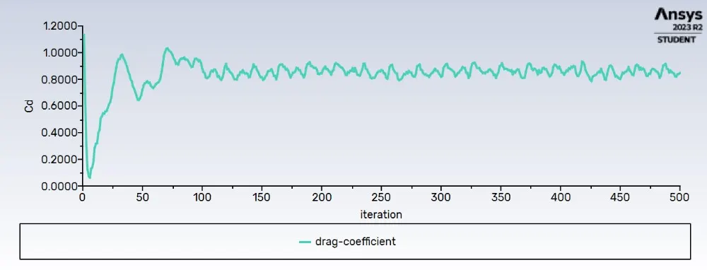
• Plots of the coefficient of lift :-
  
• If we run with Reynolds number is 10 then the lift coefficient then we will got plot like this.
• 
  
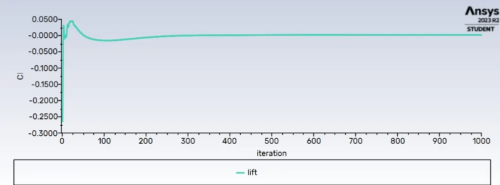
• If we run with Reynolds number is 100 then the lift coefficient then we will got plot like this.
• 
  
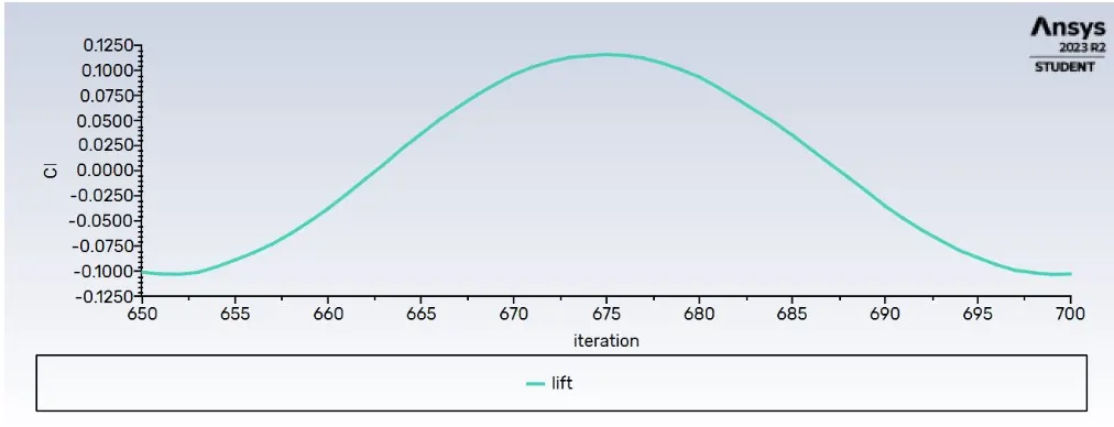
• If we run with Reynolds number is 1000 then the lift coefficient then we will got plot like this.
• 
  
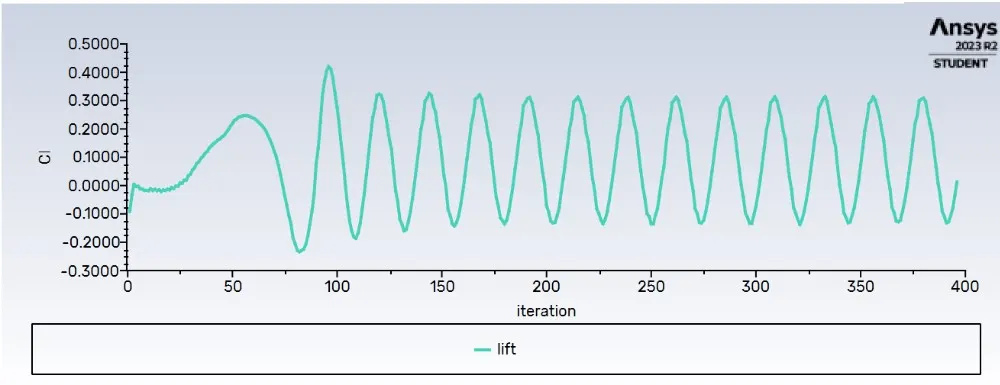
• If we run with Reynolds number is 10000 then the lift coefficient then we will got plot like this.
• 
  
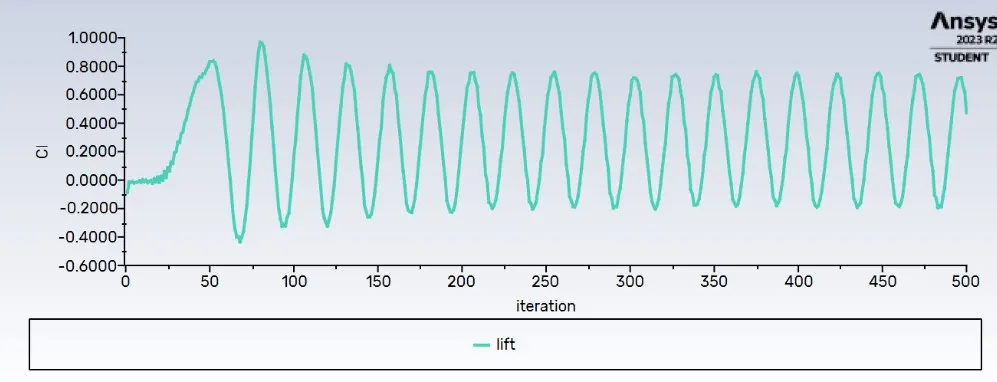
• If we run with Reynolds number is 100000 then the lift coefficient then we will got plot like this.
• 
  
• Plots to show vortex shedding behind the cylinder :-
  
• We will run after 500 time iteration then we will got this vertex shedding inside this steady state.
• 
  
• We will run after 3000 time iteration then we will got this vertex shedding inside this unsteady state.
• 
  
• Mention the referred material :-
  
• 
  
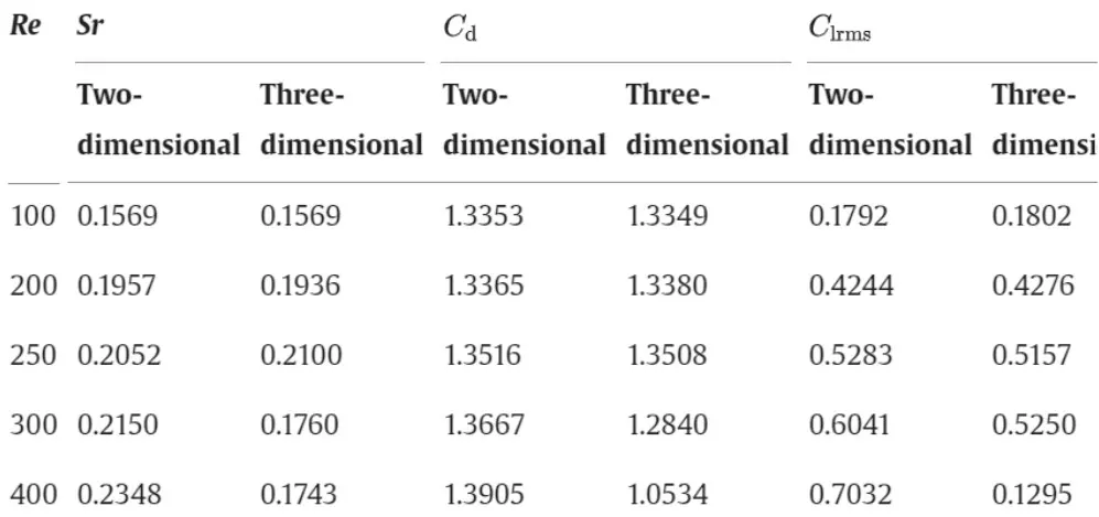
• If we run with Reynolds number is 100 then the drag coefficient value is 1.3301 . In this Reynolds number , we will got good result inside the steady state.
• If we run more then 3000 then the monitor point is going to be fluctuating with same ratio and we have to check the monitor point when its going to converge then we have to stop the iteration. After that i got drag coefficient is 0.1359 and Strouhal number is 0.157 . It give us good result as compare to unsteady state.

---