Week 2 - Flow over a Cylinder.
part-1
Steady case:
In this project, we started to create a model first we opened a space claim, and then we began to develop the geometry one by one like a cylinder and rectangle body, after completing the geometry we used the pull tool and we saw suddenly it's changed to the surface then we select the select tool then we deleted inside the cylinder after that we are going for next meshing part, then we closed the geometry section we opened the meshing part we clicked on mesh then we have seen basic quadrilateral mesh, so we need triangular mesh than we right clicked on mesh then we clicked on insert method after that we clicked on geometry then we clicked on the face and we selected the full face then we have seen it's showing one body. Then we changed the method of quadrilateral mesh to the triangle method. After that, we clicked on mesh and clicked on generated mesh, then we saw that our mesh was a triangle then we changed the element size to 0.25, and again we generated mesh then we got a good mesh count. After that, we saw our circle was not perfect, and sharp corners were there that would affect the flow, So we wanted to insert a sizing method then we selected the edge and applied the type we changed to the number of divisions, and we put the number of divisions 36, After that we clicked on generate a mesh and we got smother mesh. Then we insert the inflation layer after that in geometry we select the body and in boundary we select the edge in the inflation option we choose the first layer thickness and then in inflation height we put 5e-3. Then in the inflation layer, we changed to 6. After that, we clicked on generate the mesh. Then we assigned the inlet and outlet and then the next walls and last ones is symmetry.
Next, we went for a setup, while opening setup we used solver 4 and double-precision, and then we opened the setup, after opening we checked the mesh, so our mesh is perfectly fine. Then we checked our boundary conditions and everything was good. Next, we are going to set up physics steady state analysis and then a pressure-based solver after that, the viscous model is laminar, and we are going to material and then open a fluent database next we type air and copy that air then we rename the user-material then we closed did. then we deleted unwanted material and next, we went to properties then we changed densities to 1 and viscosity to 0.02. then down click on changed and closed.
Next, we are going to set up the boundary condition. In that one inlet, the velocity magnitude is changed to 1 m/s, and the outlet pressure is 0 pascal. Then in the wall, we are using a no-slip boundary condition.
Next, we went for the solving process we clicked on the definitions, and then we used a new surface report then we used vertex average then we changed the name monitor-point but we did not create a monitor point so we went to post-processing then we clicked on the surface then we clicked on point and we make a point there so in options selected point then x0 is 10(m) and y0 is 0(m) and name we are changing to monitor-point. then we went for the solving process we clicked on the definitions, then we used a new surface report then we used vertex average then we changed the name monitor-point-velocity, and then the field variable is velocity then we selected monitor-point, and then we clicked ok.
Next, we use the Hybrid method and then we initialize the solution next we go to post-processing in contour we change the name velocity and in the option we use filled, and then we select everything and contours of we change to velocity then we click on save/display. then we click on compute, and we see our initial value. Then again we click on the contour and this time we are looking at the pressure then we change the contours of the pressure, then in the option we select the filled option we select all components click on save/display, and then compute. so we see our pressure is 0. This is only our initial condition.
Next, we are again back to solving in that one setting we changed to a simple then opened residual and we unchecked the convergence then clicked on ok . then we put our no. of iteration 500. After that, we clicked on calculate, and we saw our monitor point velocity and scaled residuals also appearing after that, we saw our Flutchion started, and then we showed velocity display, we took our first steady state for that one we took,
1. Reynolds Number 100.
2. Velocity- 1
3. Viscosity- 0.2
4. Density- 1
5. Area-2
First, we got scaled residuals 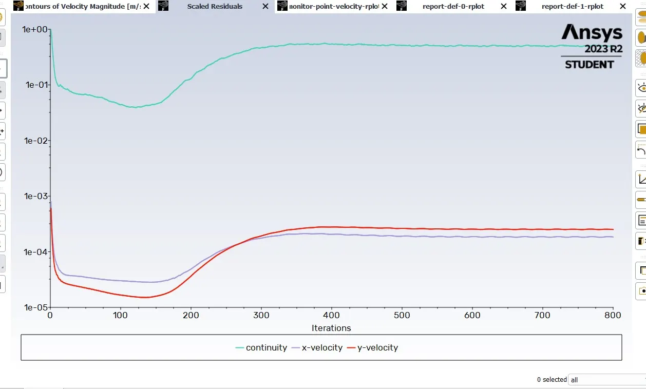
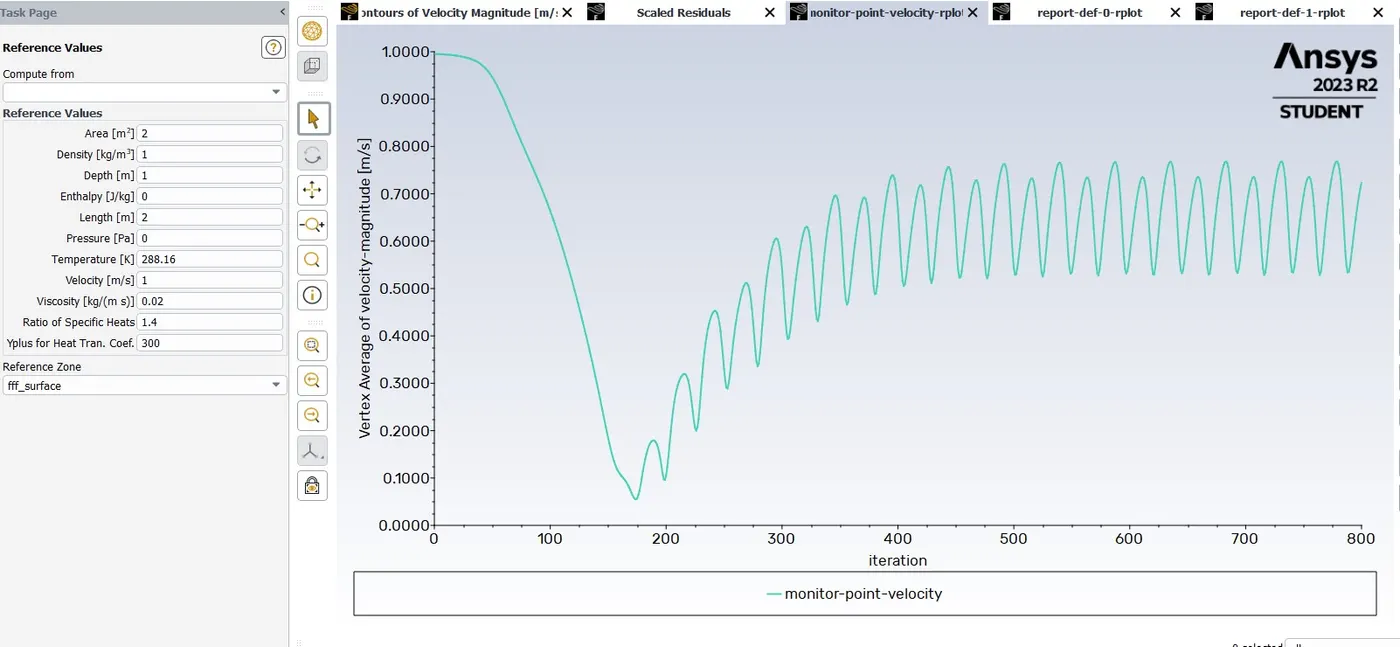
Then next we are going to monitor point velocity, here the fluctuation is continuously fluctuating, and after the run of some iterations, the function is converged.
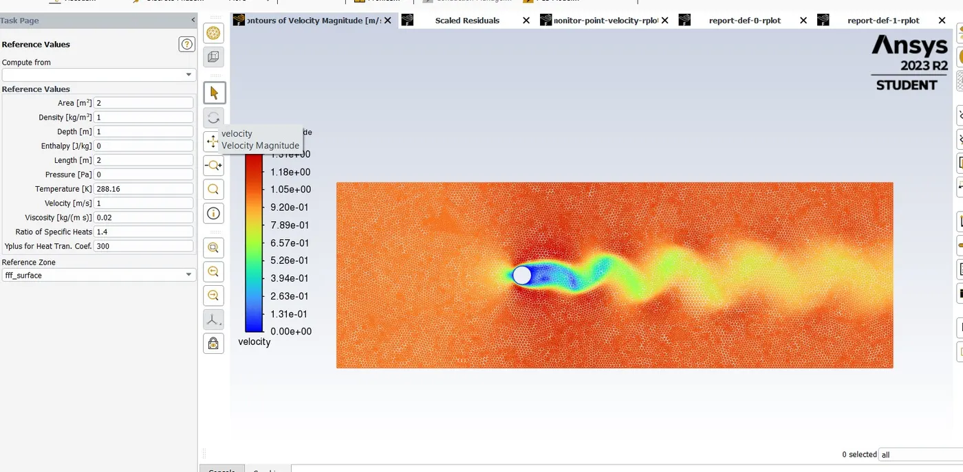
Next, we are going with velocity magnitude, here seen after some periodic time the fluctuation continuously going on smoothly for converged.
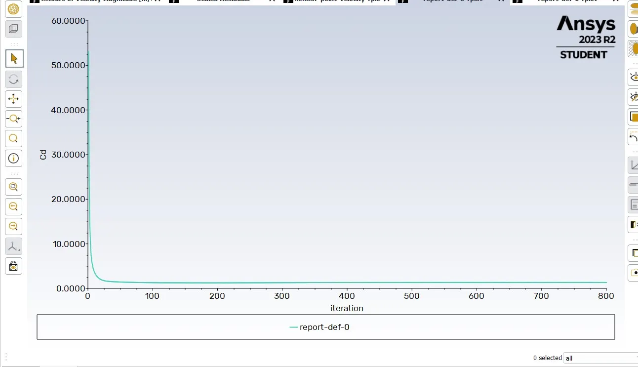
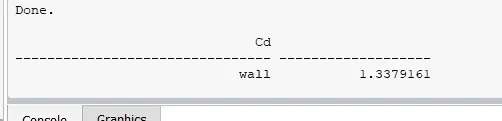
Next, the coefficient of drag flow comes at the point around 1.33 then it goes straight.
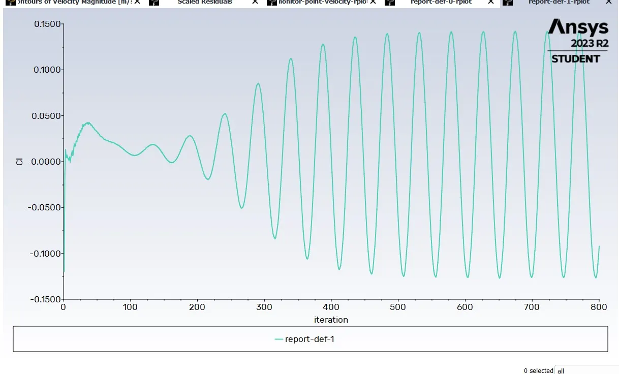
Next, we are going with the coefficient of lift, here we can see the flow is coming at a point then it starts fluctuating for the normal path.
Expected results:
1. In the first case flow has converged. we got all the plots.
2. We have shown plots of the coefficient drag and lift in above.
3. Above we show the vortex shedding behind the cylinder.
Unsteady case:
In the unsteady case directly we are going to set up physics unsteady/Transient state analysis and then a pressure-based solver after that, the viscous model is laminar. then next, we check all the Reference values whatever we put in steady case we see everything is there. Next, we use the Hybrid method and then we initialize the solution next we go to post-processing, after that, we put time steps size 0.001, and no of the steps 500 then we calculate. Then we see our solution is converged first we are going with scaled residuals.
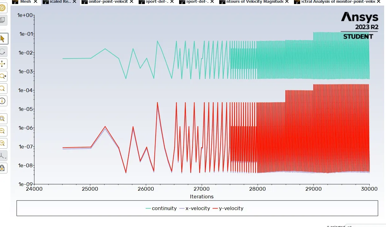
here we see our solution has converged it started with a little bit slow then slowly it is converged.
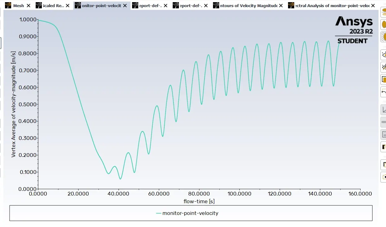
Here we can see first our vortex shedding starts at 1.0000 then it gradually goes down then its one position starts fluctuating after that its fluctuation is continuously going then it converged.
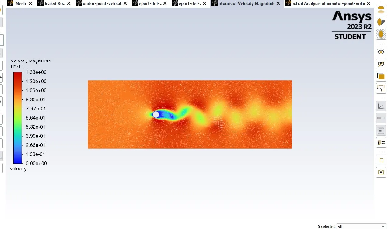
Here velocity magnitude first starts with a slow little bit after some time flow starts to fluctuate then it converged.
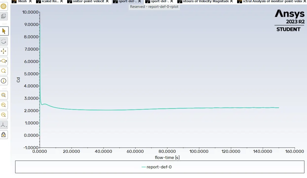
Here when see our solution is converged then we get our coefficient drag value is around 1.3142.
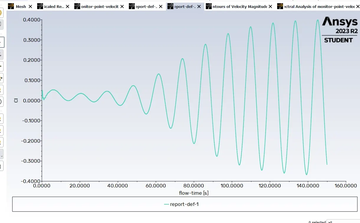
Next, we are going with the coefficient of lift, here we can see the flow is coming at a point then it starts fluctuating for the normal path.
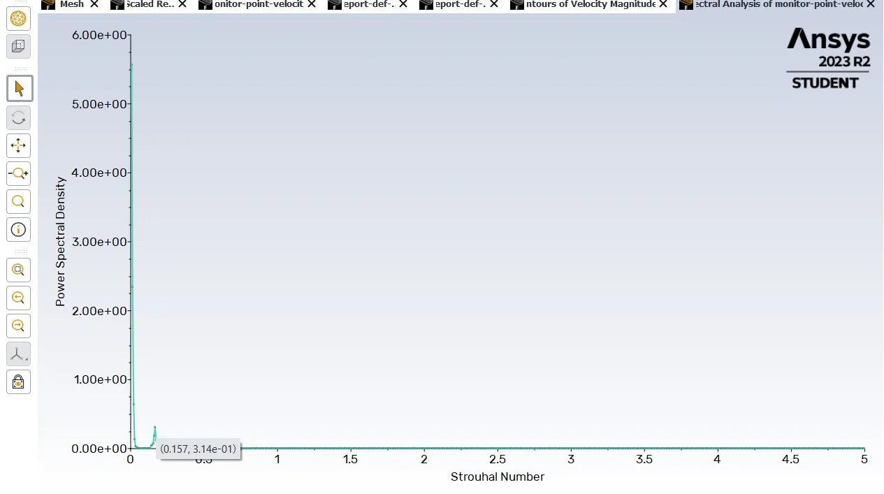
Here, when see our solution is converged then we get our strouhal number for Re-100 is 0.157.
Expected results:
1. In the Second case flow has converged. we got all the plots.
2. We have shown plots of the coefficient drag and lift in above.
3. Above we show the vortex shedding behind the cylinder.
Part-2
2)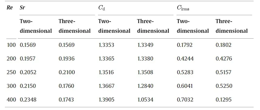
In the above, we see our coefficient drag we got 1.3379 and as per reference, they have given 1.3353, so here around it matches with the reference literature and also error within 5%, and another one strouhal number we got 0.157, and as per reference value 0.1569, so here also error within 5%.
part-2
1) Next we are going to calculate the Reynolds number 10, so for that one we duplicate the project then we directly open our setup then next we change only our Renyold number so for that one we need to change the reference value
1. Reynolds Number 10
2. Velocity- 1
3. Viscosity- 0.2
4. Density- 1
5. Area-2
Then we initialize after that we are given 500 iterations then we see our solution is not converged so again we are given 500 iterations still the same path is showing. so after the 2000 iteration, the solution is not converged.
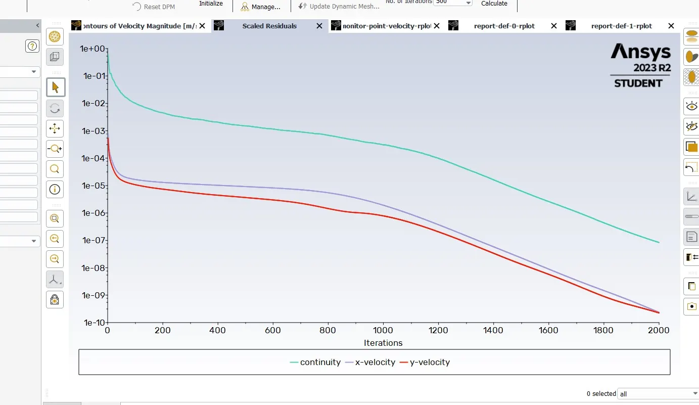
First, we can see our scaled residuals gradually decreasing but it is not converged. so due to our Reynolds number being 10. so it is not converged properly.
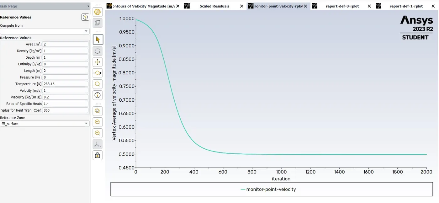
Next, we can see our vertex shedding, starting at one point and then gradually decreasing and then going straight but it is not converged so that there are no changes in line.
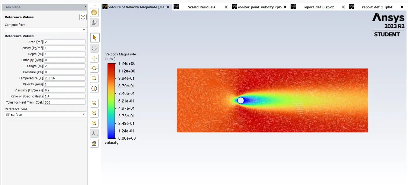
Here we can see our velocity magnitude, so there are also no changes in the path due to our Reynold number it is going straight.
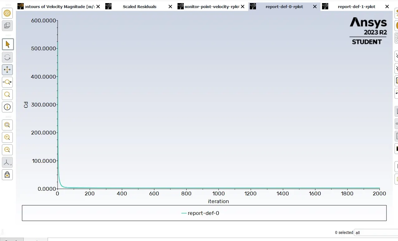
Here we can see our coefficient drag gradually decreasing and then going straight. so we got CD value is 3.3241.
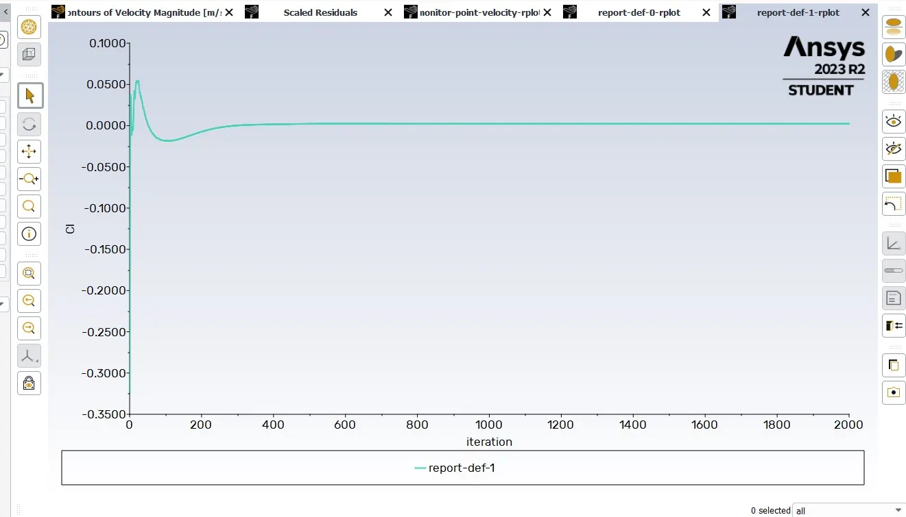
Here we can see our coefficient lift is going one pick point then it's coming a little bit down and then going straight. so we got CL value is 0.0022
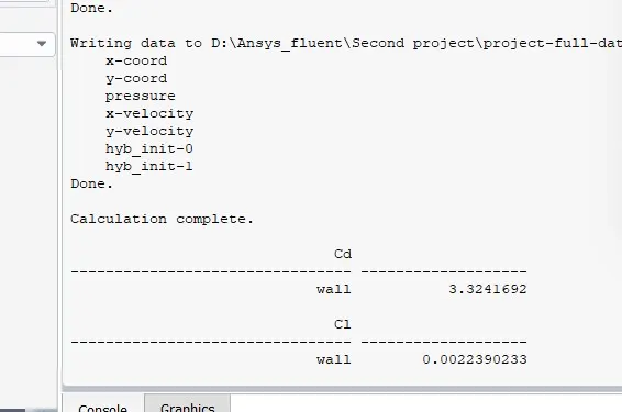
Here we can see our calculation value of CD & CL.
Next, we are going to calculate the Reynolds number 1000, so for that one, we duplicate the project then we directly open our setup then next we change only our Renyold number so for that one we need to change the reference value
1. Reynolds Number 1000
2. Velocity- 1
3. Viscosity- 0.002
4. Density- 1
5. Area-2
Then we initialize after that we are given 500 iterations and we see our solution is converged.
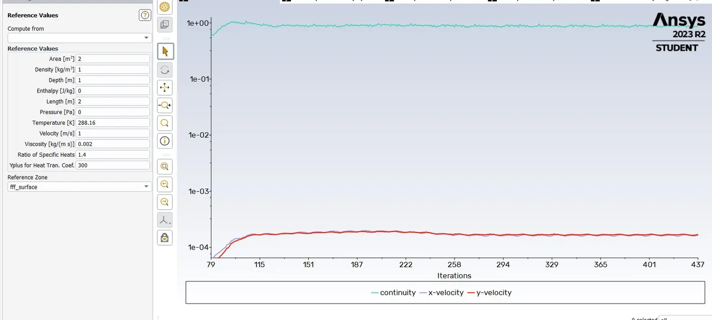
First, we can see our scaled residuals already converged and it is showing so many small fluctuations is there and it's going a single line.
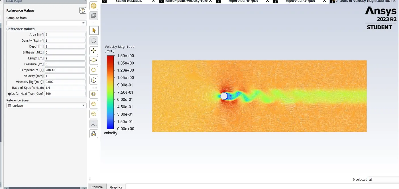
Here, we can see the velocity magnitude of the fluctuation is showing good and we see our solution is converged.
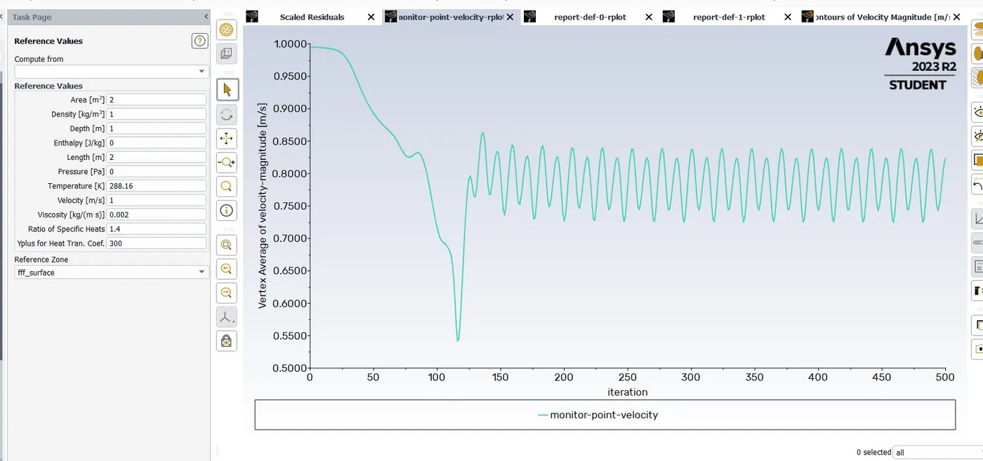
Here we can see our vertex shedding first started at a point and then gradually went down after that it went to a pick point then the fluctuation started and our solution also converged.
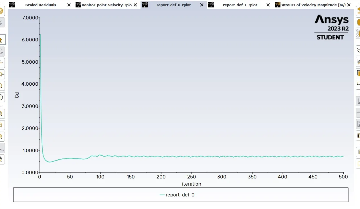
Here our solution is converged and our CD value is 0.7407.
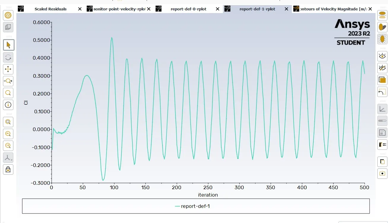
Here our solution is converged and our Cl value is 0.3117.
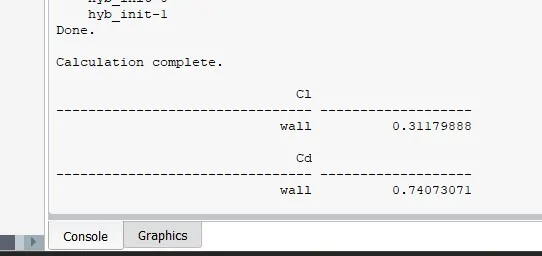
Here we can see our calculation value of CD & CL.
Next, we are going to calculate the Reynolds number 10000, so for that one, we duplicate the project then we directly open our setup then next we change only our Renyold number so for that one we need to change the reference value
1. Reynolds Number 10000
2. Velocity- 1
3. Viscosity- 0.0002
4. Density- 1
5. Area-2
Then we initialize after that we are given 500 iterations and we see our solution is converged.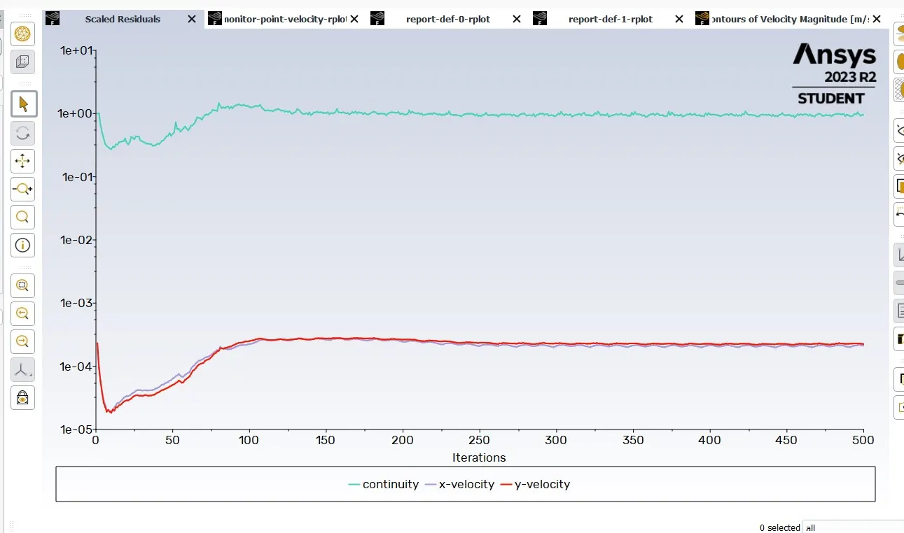
First, we can see our scaled residuals already converged and it is showing so many small fluctuations is there and it's going a single line.
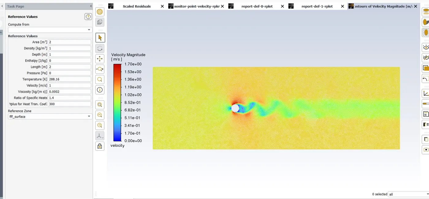
Here, we can see the velocity magnitude of the fluctuation is showing good and we see our solution is converged.
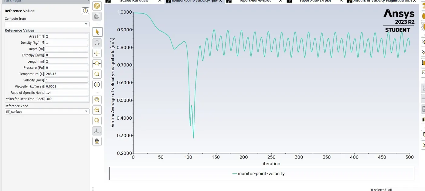
Here we can see our vertex shedding first started at a point and then gradually went down after that we saw one small fluctuation then again went to a pick point then the fluctuation started and our solution also converged.
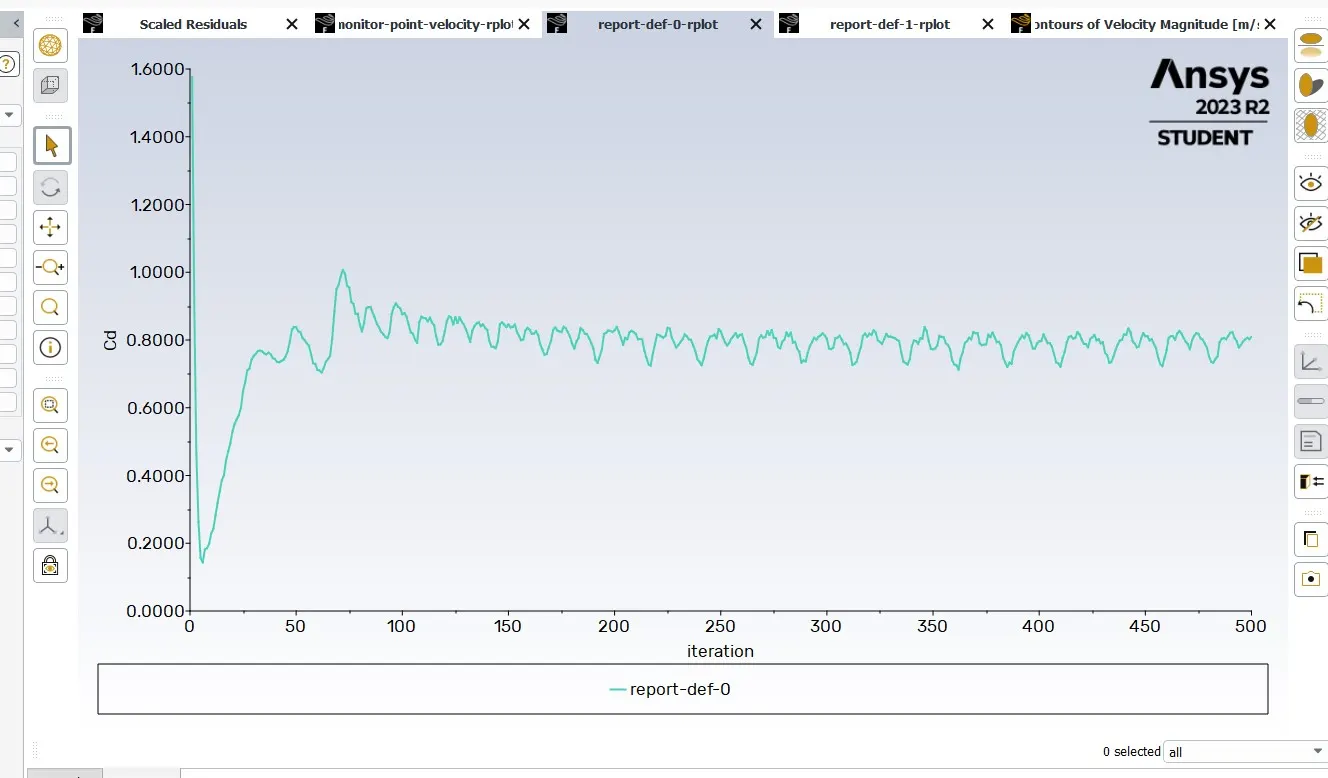
Here our solution is converged and our CD value is 0.4735.
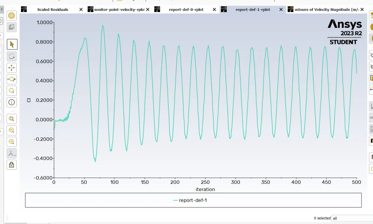
Here our solution is converged and our Cl value is 0.8092.
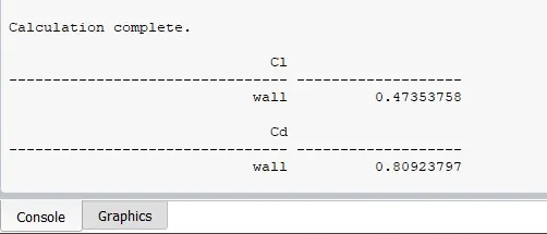
Here we can see our calculation value of CD & CL.
Next, we are going to calculate the Reynolds number 100000, so for that one, we duplicate the project then we directly open our setup then next we change only our Renyold number so for that one we need to change the reference value
1. Reynolds Number 100000
2. Velocity- 1
3. Viscosity- 0.00002
4. Density- 1
5. Area-2
Then we initialize after that we are given 500 iterations and we see our solution is converged.
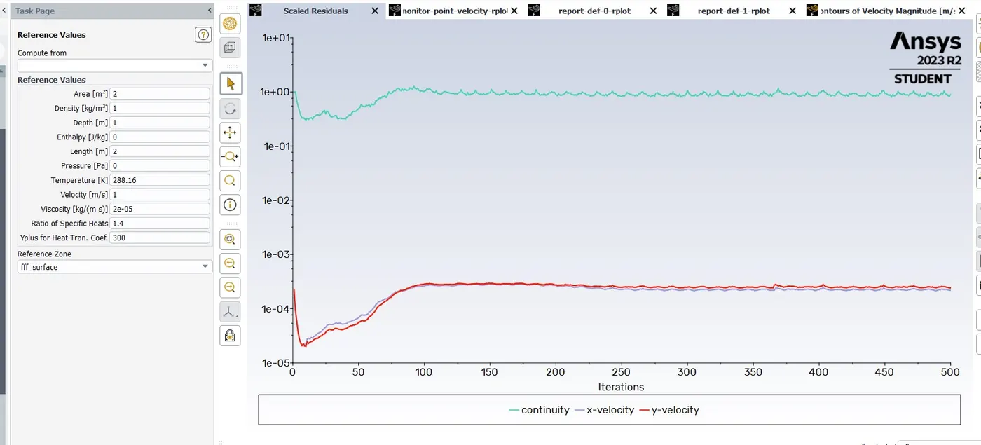
First, we can see our scaled residuals already converged and it is showing so many small fluctuations is there and it's going a single line.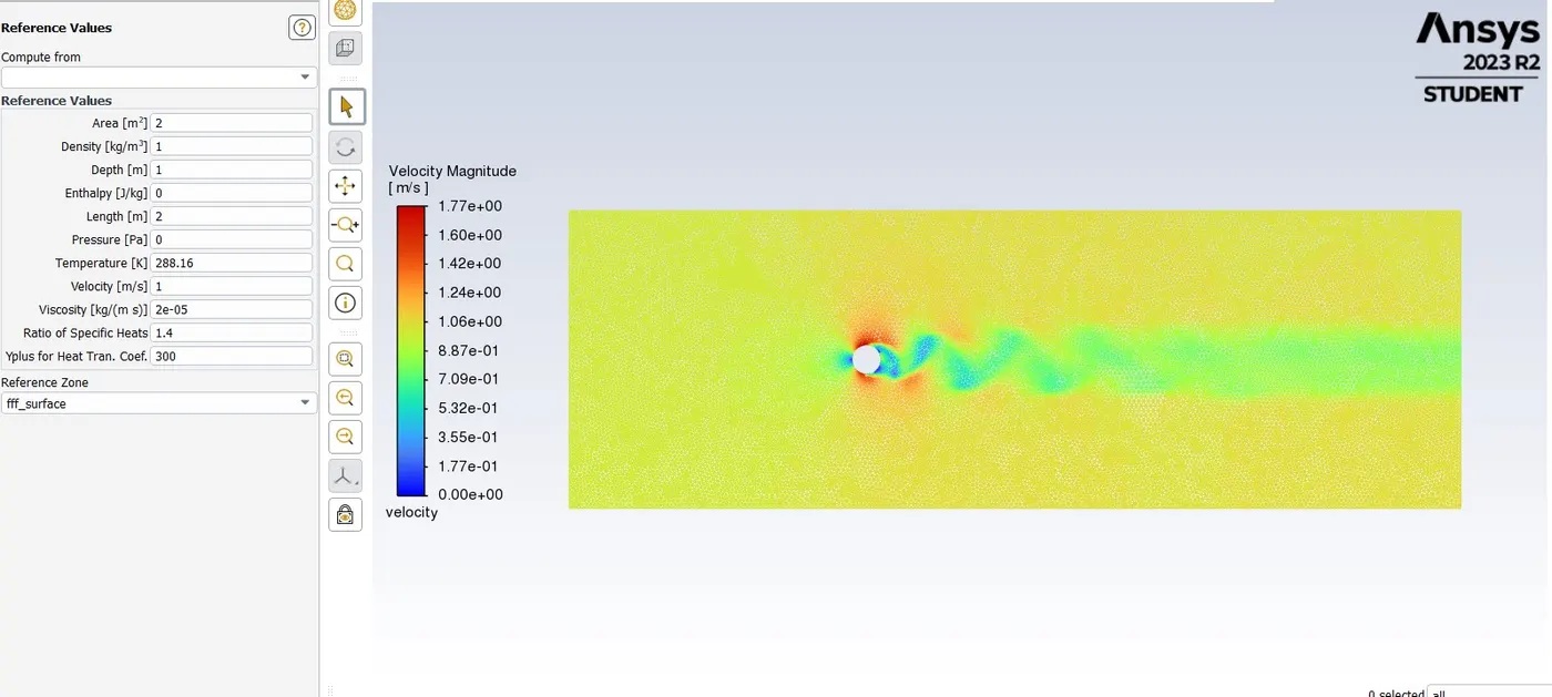
Here, we can see the velocity magnitude of the fluctuation is showing good and we see our solution is converged.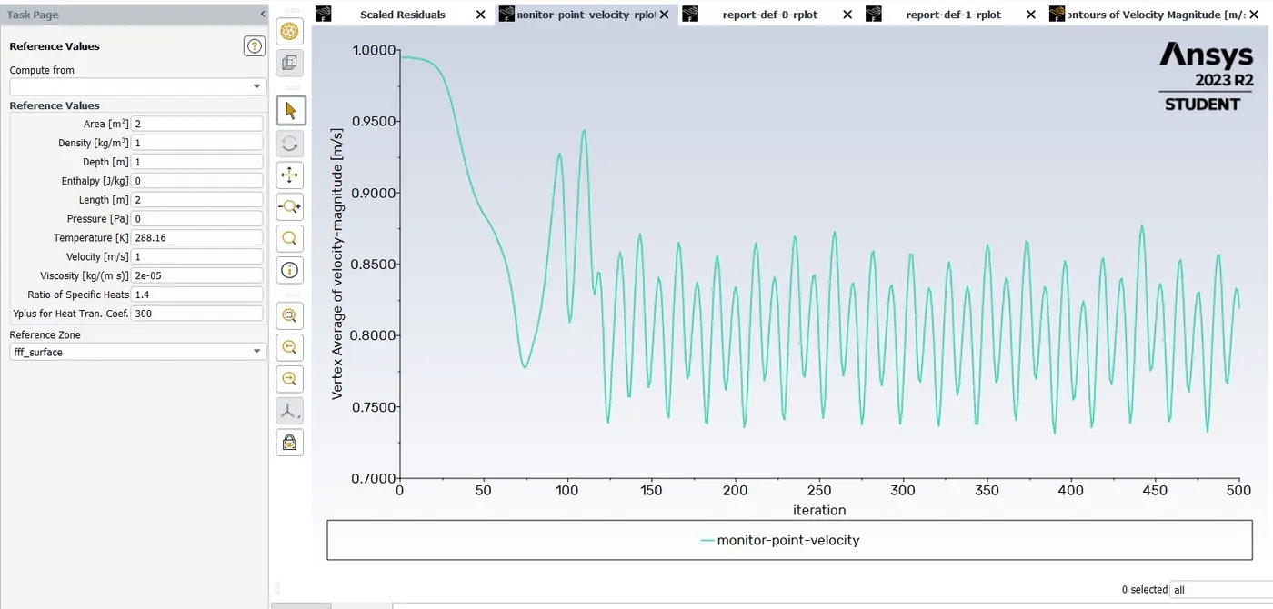
Here we can see our vertex shedding first started at a point and then gradually went down after that it went to a pick point then the fluctuation started and our solution also converged.
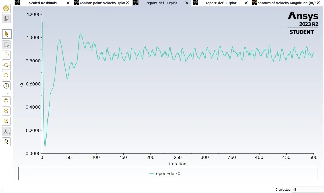
Here our solution is converged and our CD value is 0.1731.
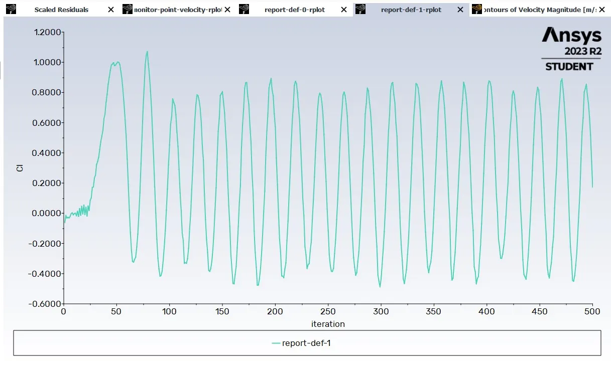
Here our solution is converged and our Cl value is 0.8648.
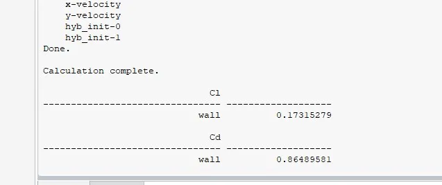
Here we can see our calculation value of CD & CL.
The referred material author R.K. Bansal.