Numerical Analysis and Simulation of Flow Past a Cylinder: Effect of Reynolds Number on Drag Coefficient and Flow Characteristics.
Aim: To simulate flow past a cylinder with varying Reynolds number and interpret the flow characteristics.
Objectives:
1. Simulate the steady and unsteady (transient) cases for range of Reynolds number.
2. To calculate the drag and lift coefficients for the respective cases.
3. To calculate strouhal number for unsteady case.
4. To visualize Von Karman Vortex Shedding and understand the phenomenon.
5. To Validate drag coefficient with standard research paper.
Methodology:
In this project, the flow past a cylinder is simulated and post-processed in Ansys Fluent. Initially, under laminar flow conditions the steady state simulation is carried out at a Reynold's number of 100. Accordingly, unsteady (transient) simulation is executed at the respective Reynold's number. The strouhal number is calculatd for unsteady case, drag and lift coefficients are calculated for both the cases. At such Reynold's number, Von Karman Vortex Shedding is visualized and understood. Then at different Reynold's number, steady state simulations are set-up to visualize vortex shedding and the effect on drag and lift coefficients.
Introduction:
The flow past a cylinder is a classical case in fluid dynamics to study external flows over a blunt body. The flow pattern and drag on the cylinder are functions of Reynolds number (`Re = (rhoVD)/mu`), based on the cylinder diameter 'D' and the undisturbed free stream velocity 'V'. The flow pattern at high Reynolds number (`Re_(D) > 10000`) is sketched in fig 1(a) and 1(b).
- At the leading edge of the cylinder a stagnation point is formed where the oncoming flow is at rest. The pressure at this point is called as stagnation pressure.
- To the either side of the stagnation point the flow accelerates around the forward suface of the cylinder producing drop in pressure.
- Immediately adjacent to the cylinder surface a thin boundary layer is formed.
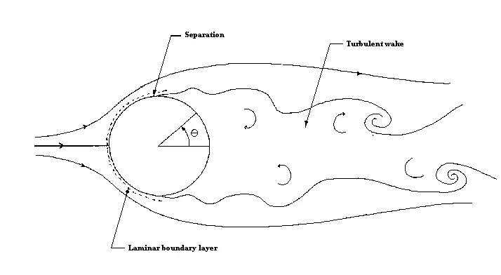
Fig 1(a): Sub-critical Reynolds number
- At low Reynolds number (generally less than 400000 (it depends upon the shape of the body and free stream velocities for external flow cases) the boundary layer remains laminar from the stagnation point at the front of the cylinder to the point where it separates.
- The resulting flow pattern (fig 1(a)) termed as sub-critical is associated with high drag on the cylinder.
- In this flow pattern there is no transitioning to turbulent boundary layer.
- Due to adverse pressure gradients the laminar boundary detaches from the flow and flow separation takes place (Laminar boundary layer possess lesser momentum and is easily influenced by adverse pressure gradients).
- Downstream of separation the flow quickly becomes turbulent and a broad wake is formed. The wake as whole is unstable and rolls up into vortices that are shed unsymmetrically at regular intervals from the cylinder. This type of wake is called as Karman vortex street.
- Because of separation the pressure remains low and approximately constant over the rearward face of the cylinder. This causes a net imbalance of pressure forces on the cylinder, usually referred as pressure drag.
- Pressure drag accounts 90% of the total drag on the cylinder in this regime.
- The remaining 10% is due to skin friction drag (friction between the flow and the cylinder). Most skin friction drag is produced on the forward face of the cylinder where the boundary layer is thin and velocity gradients at the cylinder surface are large.
- In this low Reynolds number regime pressure drag is more significant as compared to skin-friction drag. Beacuse of this at low reynolds number more drag is resulted.
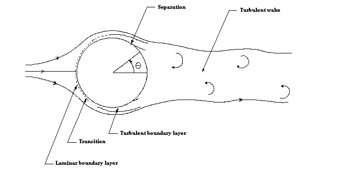
Fig 1(b): Super-critical Reynolds number
- At Reynolds number greater than the critical value (generally Re_D > 400000) the boundary layer on the forward face of the cylinder undergoes transition and becomes turbulent.
- The resulting flow pattern (fig 1(b)) termed super-critical, is associated with a much lower drag.
- The steep drop in drag (more preisely Cd (Coefficient of drag)) that occurs as a result of transition is usually referred to as drag crisis.
- The turbulent boundary layer generated in super-critial flow is much less influenced by adverse pressure gradients (turbulent flows has larger momentum to overcome adverse pressure gradients thereby leading to the flow reattachment in certain cases).
- The flow remains attached to the cylinder surface well past its maximum thickness. As a result the wake is much narrower, the imbalance of pressure forces on the cylinder surface is much smaller and the pressure drag is greatly reduced.
- This reduction in pressure drag swamps a small increase in skin-friction drag produced by the greater length of the boundary layer and its transition.
- The drag crisis need not always occur at high Reynolds number. Roughness of the cylinder surface or unsteadiness in the free-stream can cause boundary layer transition at much lower Reynolds number.
- At such high Reynolds number the pressure drag is insignificant and skin friction drag becomes more of concern.
Von karman vortex street: A von Karman vortex street is a repeatative pattern of swirling vortices, caused by a process known as vortex shedding. (Vortex shedding is an oscillating flow that takes place when fluid flows over a bluff body at certain velocities. In this flow vortices are created at the back of the body (wake region) that detach periodically from either side of the body.)
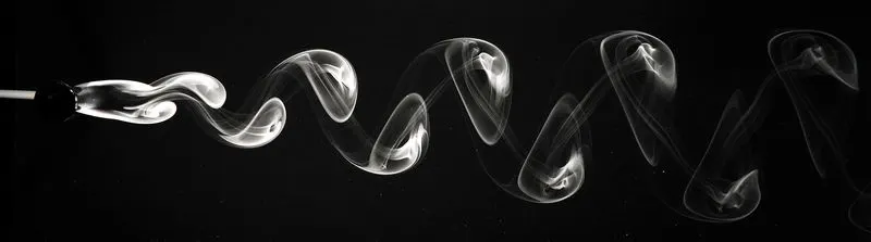
Fig 2: Vortex shedding behind the flow past a cylinder
Though vortex shedding is unsteady phenomenon occuring in laminar flows, the frequency of steady vortex shedding is observed at Re = 100. In order to calculate the frequency at which vortex are been shed, a dimensionless number called as "Strouhal number" is used.
Strouhal number:
The Strouhal number is a dimensionless value useful for analyzing oscillating unsteady fluid flow dynamics problems.
Mathematically, the strouhal number can be expressed as,
`St = (omega l) / v`
where,
`omega` = oscillation frequency
l = characteristic length
v = flow velocity
It represents a measure of the ratio of inertial forces due to unsteadiness of the flow or local acceleration to inertial forces due to changes in velocity from one point to an other in the flow field.
The Strouhal number is calculated only for transient simulations. Because of its time-accurate approximation.
Different cases to study:
In this project, different cases will be simulated and accordingly studied to understand the fundamental physics occuring in a flow past a cylinder
Part I:
In Part I, two similar cases are set-up using different type of simulation method (steady state simulations and transient simulations) with same Reynolds number.
| Cases | Reynolds Number |
| Steady state simulations | 100 |
| Unsteady (Transient) simulations | 100 |
Part II
In Part II, steady state simulations will be used for different cases which vary with the Reynolds number.
| Cases (Steady state simulations at different Reynold's number) | Velocity of the fluid (m/sec) |
| Re = 10 | 0.25 |
| Re = 100 | 2.5 |
| Re = 1000 | 25 |
| Re = 10000 | 250 |
| Re = 100000 (0.1 Million) | 2500 |
Initially cylinder geometry is created in Spaceclaim and appropriate flow volume region is defined as a surrounding to a cylinder. Moreover, in this project two-dimensional flow analysis is done and accordingly set-up is developed.
Fluid characteristics:
An artificial fluid is created to visualize the viscous flow over a cylinder. The flow will remain incompressible and viscosity will remain constant for all the cases. To attain desired Reynolds number, velocity will be modified for the respective cases.
| Density | 1 kg/`m^3` |
| Viscosity | 0.05 kg/m-s |
Other set-up characteristics:
Monitor point: The monitor point is a point in space at which flow quantities can be approximated. In this particular case, 4*Diameter = 4*2 = 8m at which monitor point is specified.
Pressure-velocity coupling method: SIMPLE (Semi-Implicit Method for Pressure Linked Equations)
Geometrical dimensions:
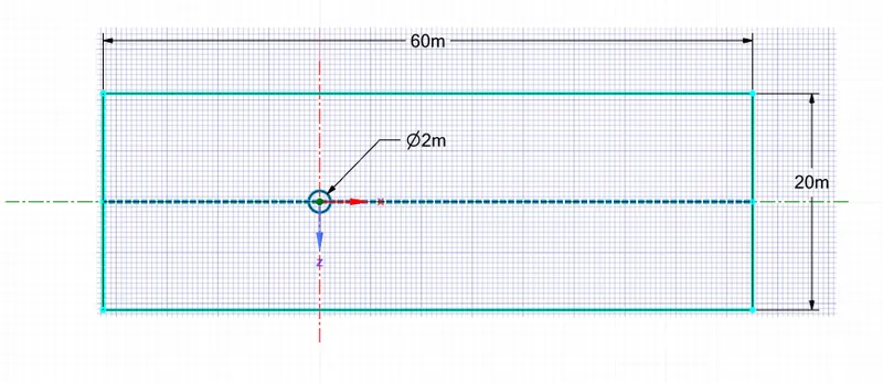
Geometry:
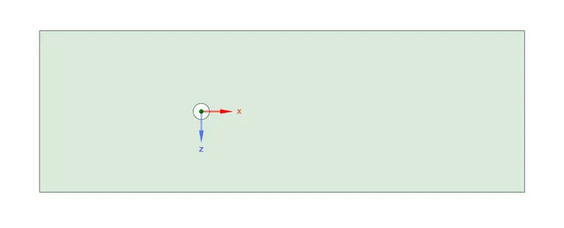
Mesh generation:
1. Mesh method:
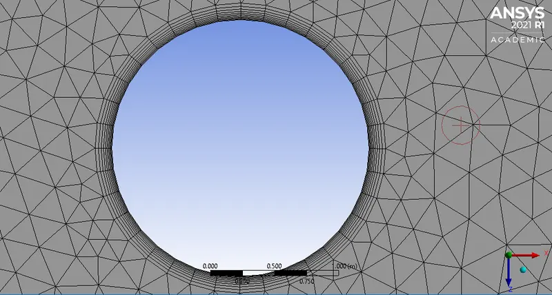
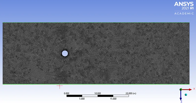
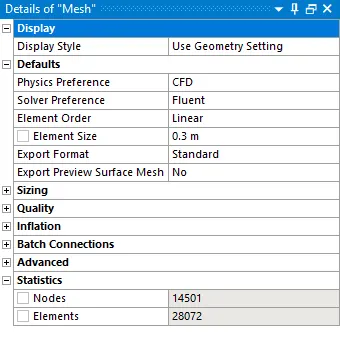
The method of meshing is selected to be as "All triangles method", which generates the triangular mesh (2-d) all over the domain. The element size is automatically adjusted by fluent (coarse mesh far away from the flow field and fine mesh towards the cylinder geometry).
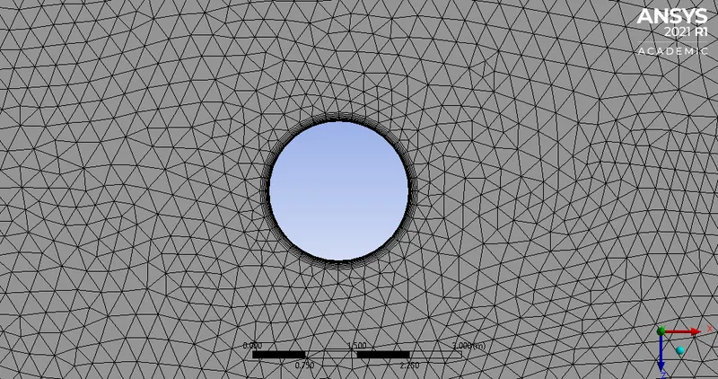
2. Sizing:
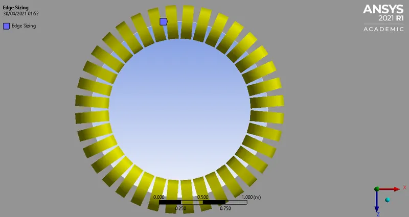
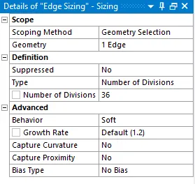
In automatic mesh generation, cylinder boundary is affected resulting in non-circular wall at the boundaries. Because of this the flow field calculation and analysis gets affected drastically. In order to avoid this, edge is sized by using number of divisions of 36 (for every `10^0`, there would be a edge and all add up to `360^0` that is nothing but circular orientation).
3. Inflation:
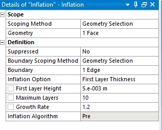
Inflation is an important aspect in meshing the geometry to capture the flow field at the wall conditons. The mesh generated using inflation is "body fitted mesh" which adapts according to the surface. Inflation option of "First layer thickness" is selected and first layer height of 5e-3 is defined. The total number of layers is assigned to be as 10 with the growth rate of 1.2.
4. Resulting mesh:
The element size is set to be as 0.3m which results in 28,072 elements.
Named selections:
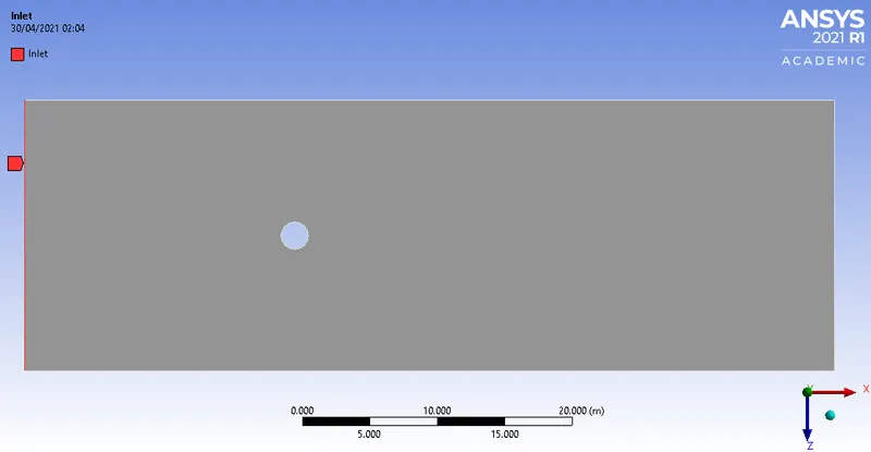
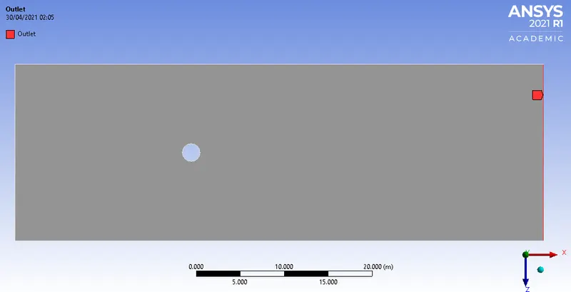
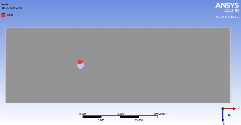
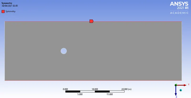
In this section, the patches of the geometry colored in red are named according the boundary conditions. Each patch is defined as the region with its respective purpose.
1. Inlet:
2. Outlet:
3. Walls (Cylinder wall):
4. Symmetry:
Part I
In this part, steady and transient simulation are executed with same Reynolds number.
A] Steady state simulation (with Re = 100)
[I] Plots:
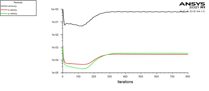
1. Residuals:
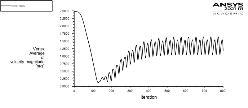
2. Velocity fluctuations at a specified monitor point:
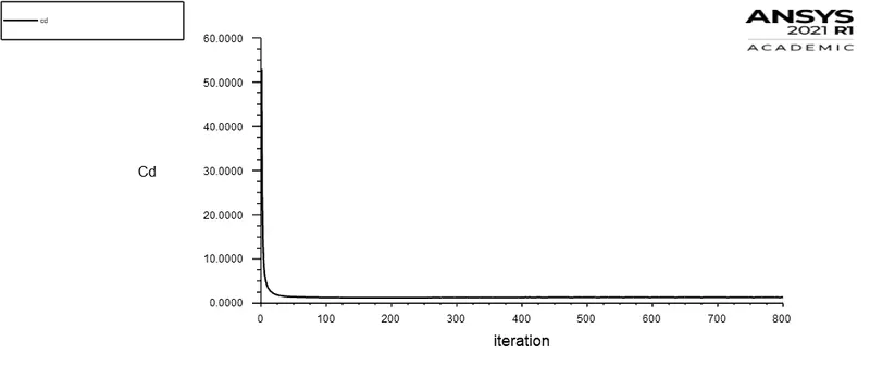
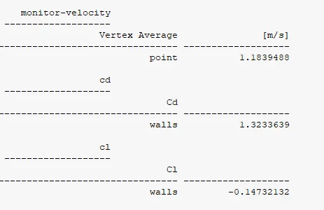
3. Coefficient of drag (cd):
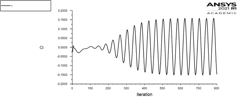
4. Coefficient of lift (cl):
Report Definitions:
[II] Contours:
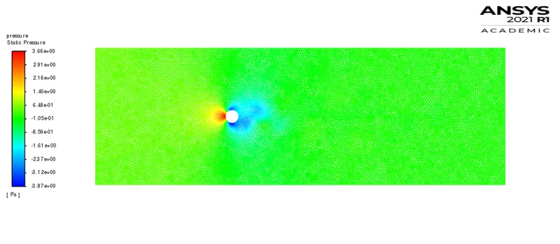
1. Pressure contour:
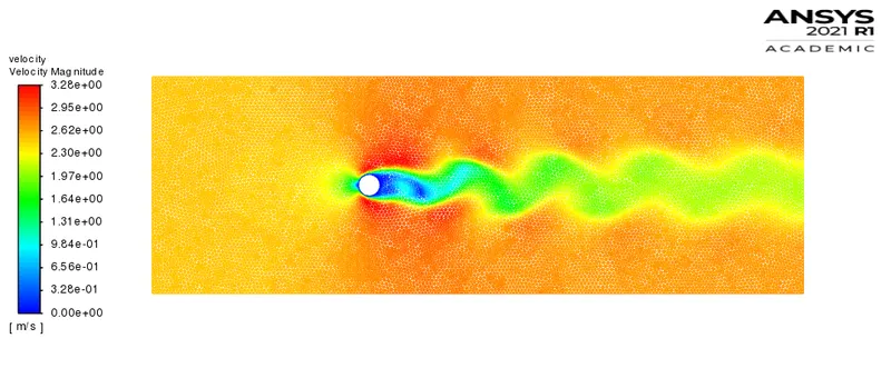
2. Velocity contour:
3. Velocity vector contour:
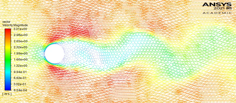
4. Velocity pathlines contour:
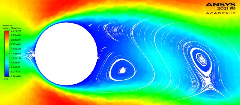
Animation:
Note: Playback speed 0.25x is suggested for proper visualization.
B] Transient simulation (with Re = 100):
Plots:
1. Residuals
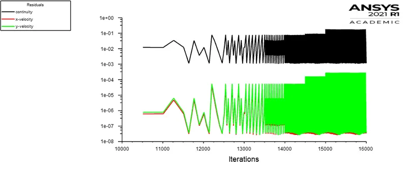
2. Velocity fluctuations at a specified monitor point:
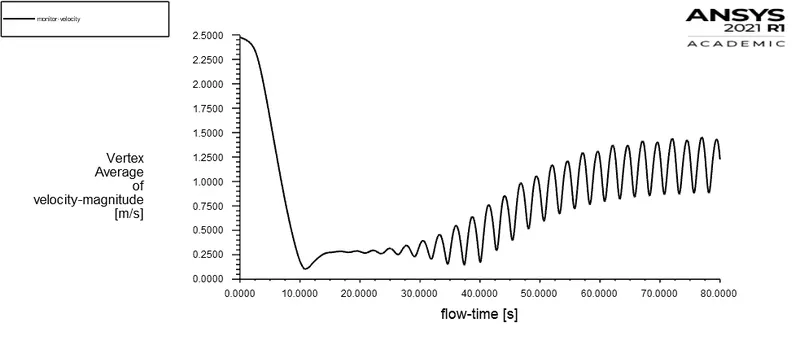
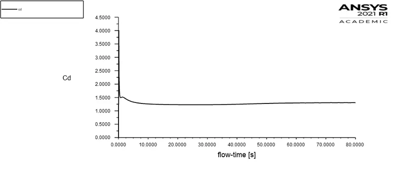
3. Coefficient of drag (cd):
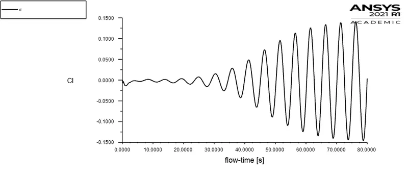
4. Coefficient of lift:
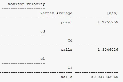
Report definitions:
[II] Contours:
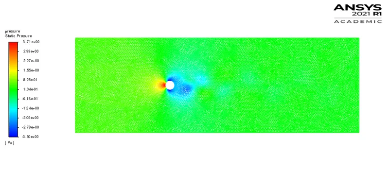
1. Pressure contour:
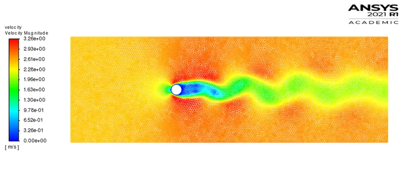
2. Velocity contour:
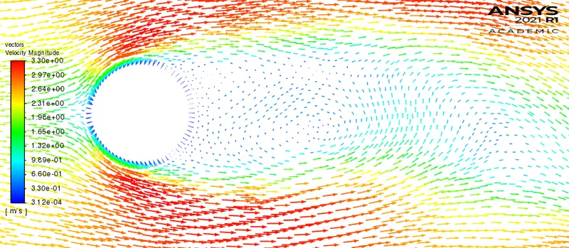
3. Velocity vector contour:
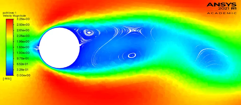
4. Velocity pathlines contour:
Animation:
Note: Playback speed 0.25x is suggested for proper visualization.
Calculation of Strouhal number:
1. Strouhal number for velocity fluctuations at a specified monitor point
`St = (omega l)/v`
l = characteristic length = 2m
v = flow velocity = 2.5m/s
`omega` = oscillation frequency = No.of cycles/time = 3/(80-70)
`omega` = 0.3
St = (0.3*2)/2.5
St = 0.24
2. Strouhal number for lift oscillations
`omega` = oscillation frequency = No.of cycles/time = 2/(80-70)
`omega` = 0.2
St = (0.2*2)/2.5
St = 0.16
Results Validation:
Strouhal number for lift coefficient:
The strouhal number as per reference standard paper [1] is 0.1569 and the resulted strouhal number in this analysis is 0.16. The results obtained in our analysis shows good agreement with standard results following the error of 3.1e-3.
Drag coefficient:
As per standard reference [1] the drag coefficient is 1.3353 and the resulted drag coefficient is 1.3046. The results obtained in this analysis are congruent with standard reference following the error of 2.3%.
Technical summary (Part I):
The steady and transient simulation gave similar results. However, as we know steady state simulation is used to get end results of a particular problem. (steady state simulations are time independent). And transient simulations are time accurate (they are time dependent) which gives results at a particular time-step. The monitor point specified above is used to identify velocity fluctuations. Both the steady and Unsteady simulations resulted in similar plots, however we cannot calculate the plot oscillations (velocity fluctuations and lift oscillations) using steady state simulation as they are not time-accurate. Therefore, it was need to opt for transient type simulations to calculate the oscillations of the velocity and lift, finally to Strouhal number. The resulted Strouhal number is 0.24 which falls in the standard range for rounded off bodies or cylindrical bodies i.e. `0.2 le St le 0.3`.
Note: Strouhal number can vary as a function of angle of attack, shape of the body, Reynolds number and other flow conditions.
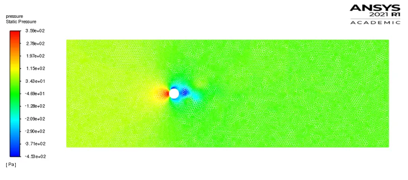
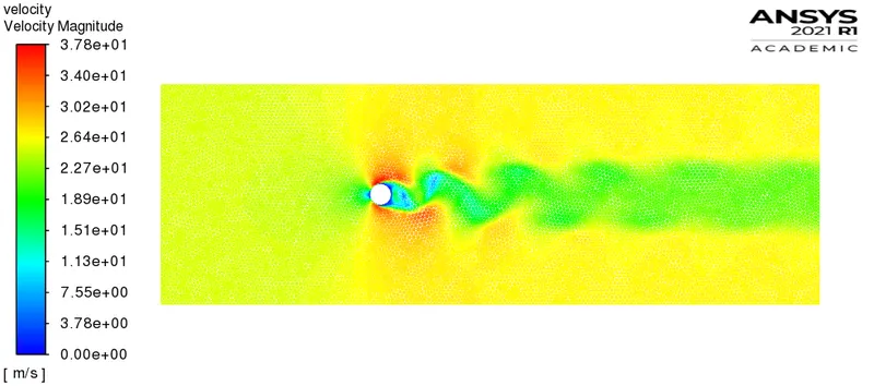
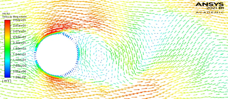
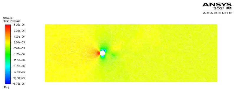
In post-processing, we see pressure at the stagnation point (forward surface of the cylinder normal to flow) is maximum and velocity is zero. There is laminar boundary layer at the forward surface of the cylinder and after certain climbing over cylinder surface, the boundary layer separates (separation point) due to presence of adverse pressure gradient. The boundary layer separation is way before the maximum thickness which leads to creation of more broader turbulent wake zone. This wake zone contributes to the low pressure region and which makes imbalance in net pressure distribution. After separation, the fluid flow struggles to flow in free-stream direction and accordingly reverses in the flow direction which leads to formation of eddies in the wake region. These eddies grow up as a function of fluid flow and shed periodically from the rearward surface of the cylinder (top and bottom) is called as Karman vortex street. Initially, the vortex shedding is unsteady but as a function of time the shedding becomes stable and steady vortex shedding is resulted. The vortex street at `90 le Re le 150` regime is laminar.
Part II:
Type of simulation: Steady
A] Reynolds number = 10
I] Plots:
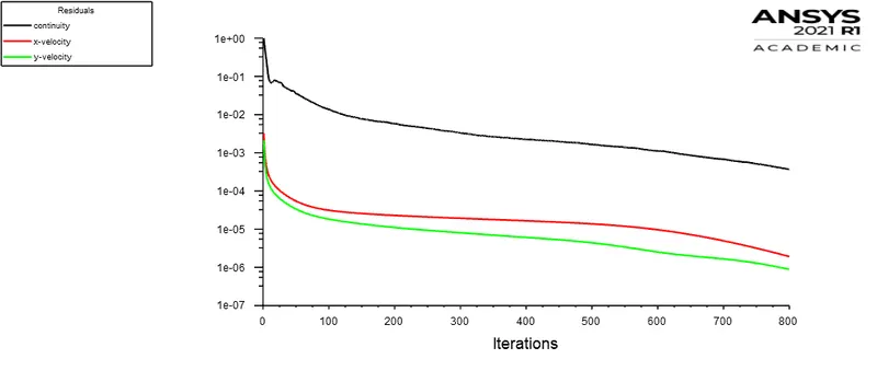
1. Residuals
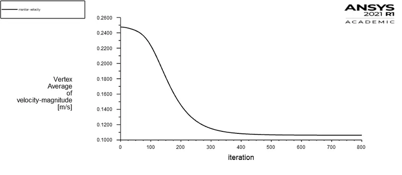
2. Velocity fluctuations at a specified monitor point:
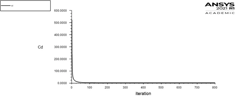
3. Coefficient of drag (cd):
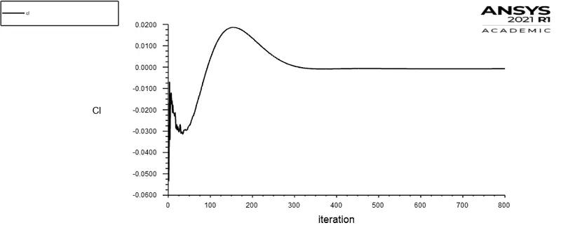
4. Coefficient of lift (cl):
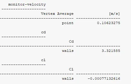
Report definitions:
II] Contours:
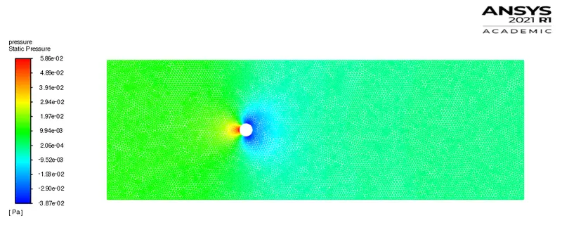
1. Pressure contour:
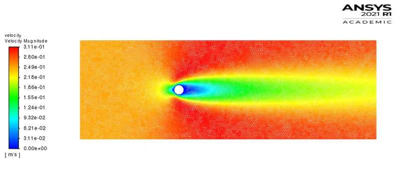
2. Velocity contour:
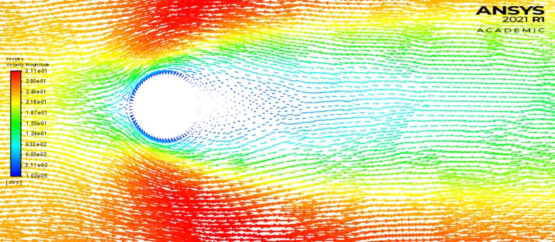
3. Velocity vector contour:
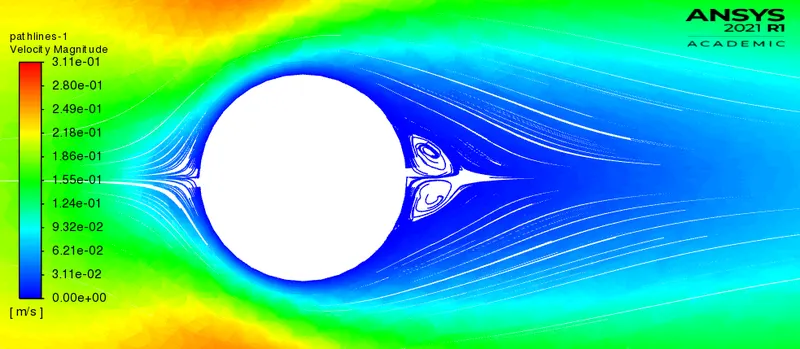
4. Velocity pathlines contour:
Animation:
Note: Playback speed of 0.25x is suggested for proper visualization.
B] Reynolds number = 1000
I] Plots:
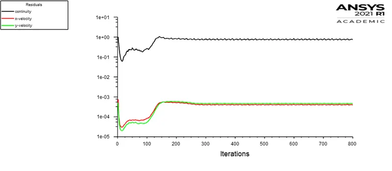
1. Residuals:
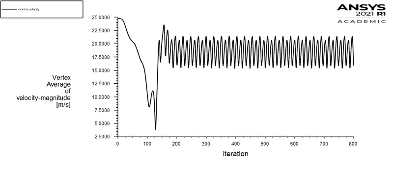
2. Velocity fluctuations at a specified monitor point:
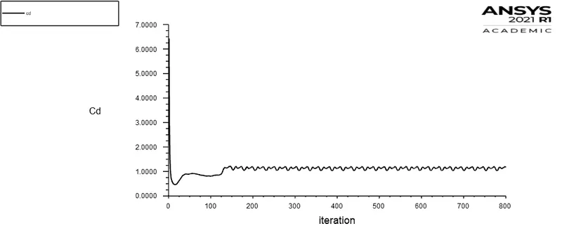
3. Coefficient of drag (cd):
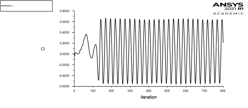
4. Coefficient of lift (cl):
Report definition:
II] Contour:
1. Pressure contour:
2. Velocity contour:
3. Velocity vector contour:
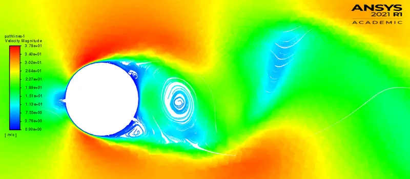
4. Velocity pathlines contour:
Animation:
Note: Playback speed of 0.25x is suggested for proper visualization.
C] Reynolds number = 10000:
I] Plots:
1. Residuals:
2. Velocity fluctuations at a specified monitor point:
3. Coefficient of drag (cd):
4. Coefficient of lift (cl):
Report definition:
II] Contours:
1. Pressure contour:
2. Velocity contour:
3. Velocity vector contour:
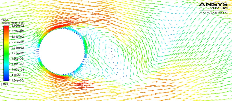
4. Velocity pathlines contour:
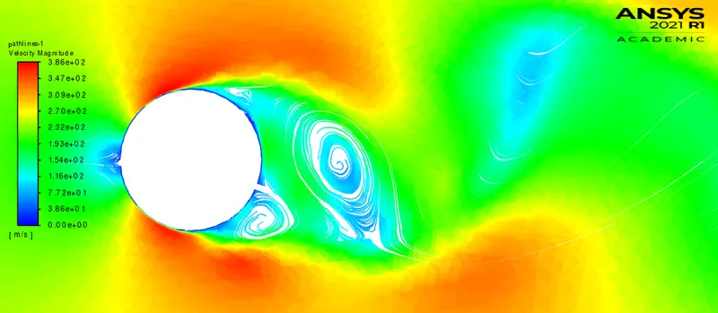
Animation:
Note: Playback speed of 0.25x is suggested for proper visualization.
D] Reynolds number = 100000:
I] Plots:
1. Residuals:
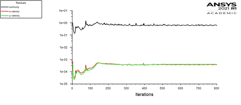
2. Velocity fluctuations at a specified monitor point:
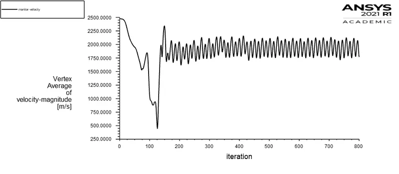
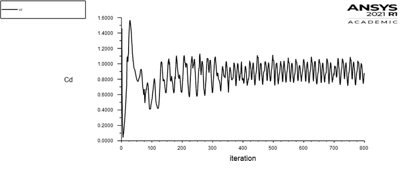
3. Coefficient of drag (cd):
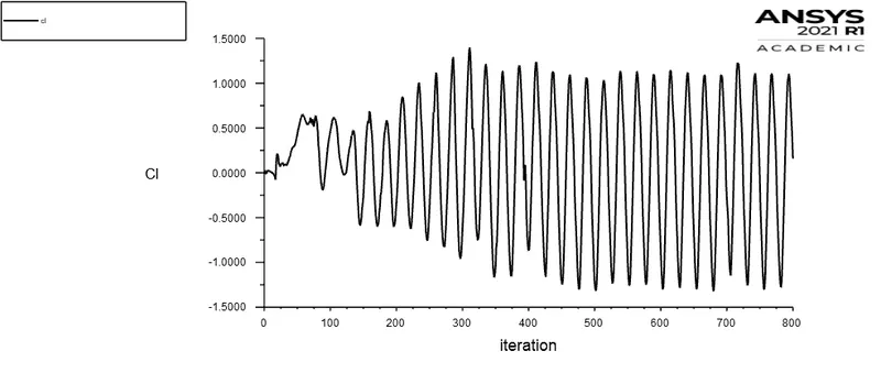
4. Coefficient of lift:
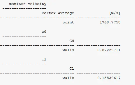
Report definition:
II] Contours:
1. Pressure contour:
2 .Velocity contour:
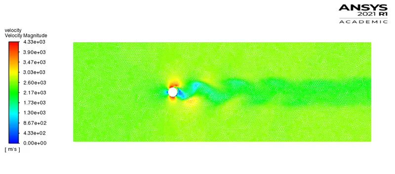
3. Velocity vector contour:
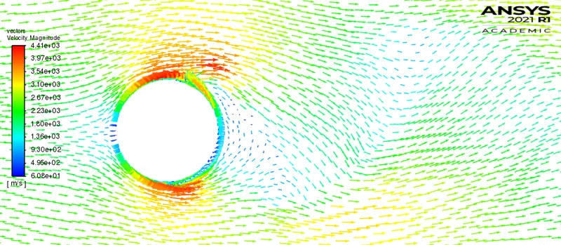
4. Velocity vector pathlines:
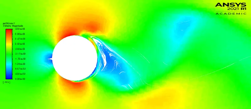
Animation:
Note: Playback speed of 0.25x is suggested for proper visualization.
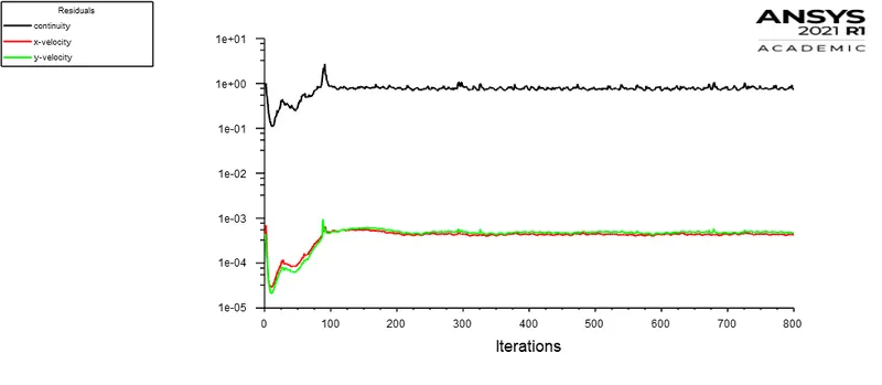
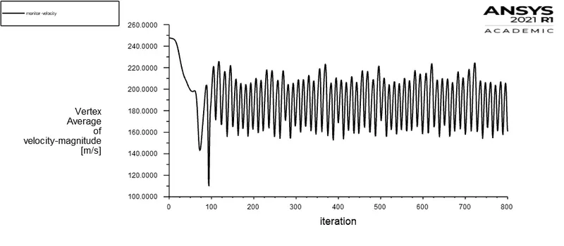
Note: In order to identify whether the flow has converged or not? We need to look upon the velocity fluctuations which are at a specified monitor point. The above presented simulation results shows the attainment of the steady velocity fluctuations. The flow quantity i.e. velocity fluctuation is monitored to identify its steady oscillation repeatation as a function of iteration / time-step. Accordingly, the plot of coefficient of drag (cd) also gives an idea about the attainment of the steady state. At this moment in time, simulation should be stopped instead consuming extensive computer resources.
Observation Table:
| Cases (Steady state simulations) | Coefficient of drag | Coefficient of lift |
| Re = 10 | 3.3215 | -0.00077 |
| Re = 100 | 1.3233 | -0.14730 |
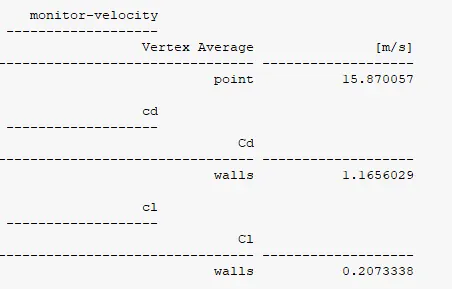
| Re = 1000 | 1.1656 | 0.20733 |
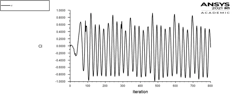
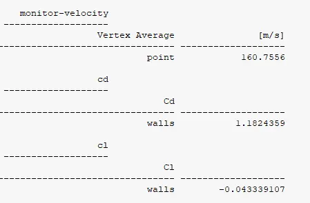
| Re = 10000 | 1.1824 | -0.04334 |
| Re = 100000 | 0.8722 | 0.15829 |
Technical summary (Part II):
Steady state simulations are used for in this numerical analysis. As transient simulation consumes extensive computation resources, as it solves the governing equation for each and every time-step. However in this analysis (Part II) the end results are more of concern as we do not intend to calculate frequency of the velocity or lift fluctuations. Instead the aim is to calculate coefficient of drag and lift. So as per the results tabulated above we can see the inverse variation of the drag with Reynolds number. The drag consists of pressure drag i.e. (due to net pressure imbalance at the rear surface of the body or wake region) and skin-friction drag (because of fluid viscous effects on the surface of the body or fluid friction).
Initially at Re = 10, the flow is attached to the cylinder forming the laminar boundary layer. The laminar boundary over the cylinder surface is responsible for viscous effects that consequently produces skin-friction drag over the surface. Accordingly, there is mild separation of boundary layer which generates small twin eddies at the rearward surface of the cylinder. These symmetric pair of vortices are fixed in the wake region which leads to reattachment of the fluid to the free-stream flow. However, the pressure distribution can be visualized in the pressure contour at Re = 10. The span of low pressure region behind the cylinder contributes to pressure drag. There is influence of both pressure drag and skin-friction drag which results in high coefficient of drag at such velocities. However at Re = 100 the wake region is lesser as compared to the flow at Re = 10, which results in comparatively less drag coefficient.
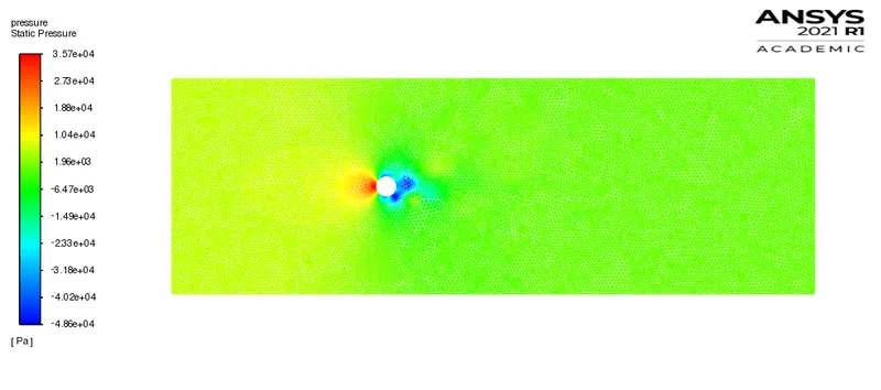
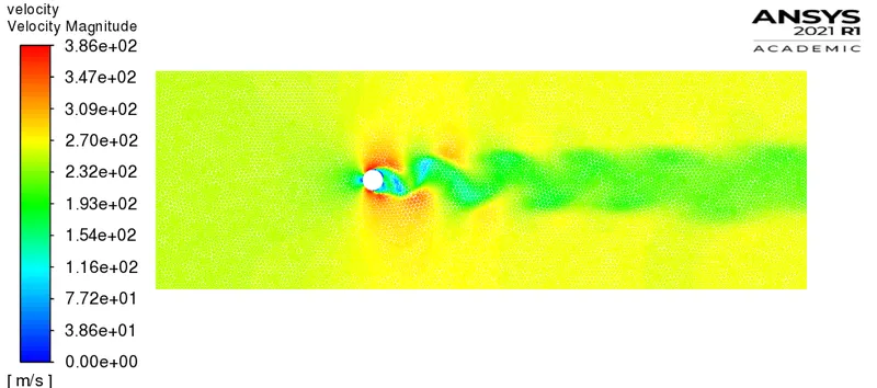
At high Reynolds number (300 < Re < 300000) there is a tranisition of laminar boundary layer to turbulent boundary layer. The turbulent boundary layer is less influened by adverse pressure gradient. Because of that the flow remain attached to the maximum thickness. The presence of turbulent boundary layer delays the separation, which results in much narrower wake at (Re = 1000, 10000, 100000) as compared to the flow at (Re = 10, 100). There is less contribution of pressure drag in such scenarios however skin-friction drag (shear drag) influences more. Vortex shedding is turbulent in this regime of Reynolds number. The eddies generated in the wake region grows up to unstable vortices due to momentum and energy transfer across the flow.
Conclusion:
The flow past a cylinder is successfully simulated and post-processed with interesting results. There is significant effect of Reynolds number over drag coefficient. The drag coefficient is significantly reduced past a increment in Reynolds number. At higher Reynolds number skin-friction drag contributes more to total drag and leads to heating of the surface, however at lesser Reynolds number pressure drag accounts for more in total drag. No general assertion can be stated over the effects of Reynolds number and drag force / coefficient as many factors like fluid viscosity, shape of the body, flow velocity, body surface roughness, aspect ratio and many more undesirable / unexplored factors contribute to it.
Generally in external flows it is prior matter of concern to delay the flow separation which results in less pressure drag over the bodies. By providing curvature or regular disruption over a bluff body generates a turbulent boundary layer over the surface which significantly reduces the total drag.
References:
1. https://www.sciencedirect.com/science/article/pii/S0307904X08000243
2. Introduction to aerodynamics by John D. Anderson