Week 2 - Flow over a Cylinder.

AIM:

To simulate the flow over a square and explain the phenomenon of Karman vortex street.

INTRODUCTION:

Two parallel rows of alternately placed vortices along the wake of an obstacle in a fluid of moderate Reynolds number. Fluid drag can be calculated from the motion of these vortices, which are stable only for a certain ratio of the width of the street to the distance between vortices along the street.Karman vortex street also called vortex trail,vortex train.

APPLICATIONS:

They occur in many engineering situations, such as bridges, skyscrapers, transmission lines, aircraft control surfaces, offshore structures, marine cables, petroleum production, pipelines, cable-laying, members of jacketed structures, and other applications.

PROCEDURE:

• Create a square with 2m diameter and an enclosure with standard dimensions in spaceclaim geometry.
• Mesh the geometry with named selections and inflation layer.
• Update and open the solver.
• Set the parameters for solving in both the cases & the setup parameters are shown below with a ss : [Case1]- Steady state , [Case2]- unsteady state
• Initialize and run the solution till it converges.
• Open results and make a velocity contour in a symmetry to view the vortex.
• Animate and save the movie to view the vortex simulations in both the cases.
• Update and save the geometry.

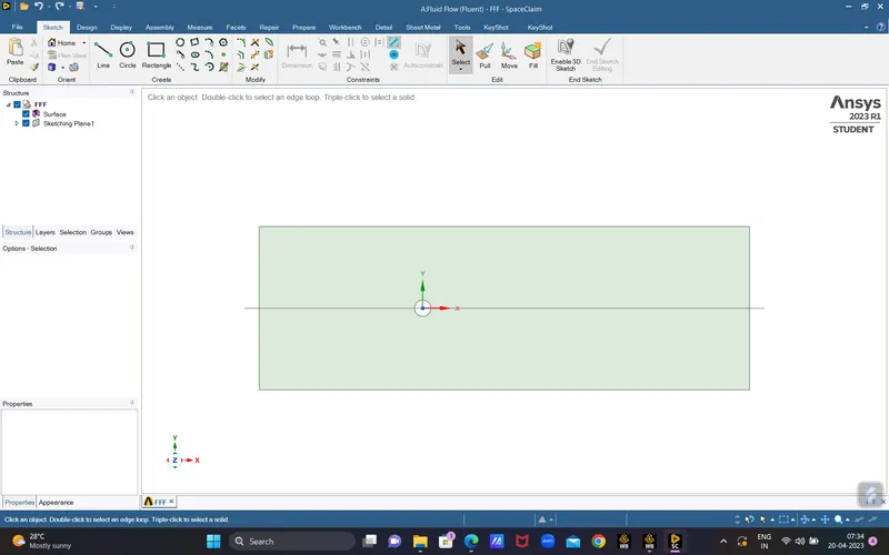
FIG 1. Geometry in spaceclaim

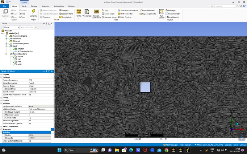
FIG 2. Meshed geometry

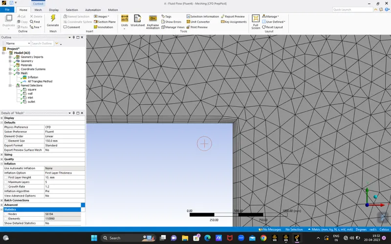
FIG 3. Inflation layers

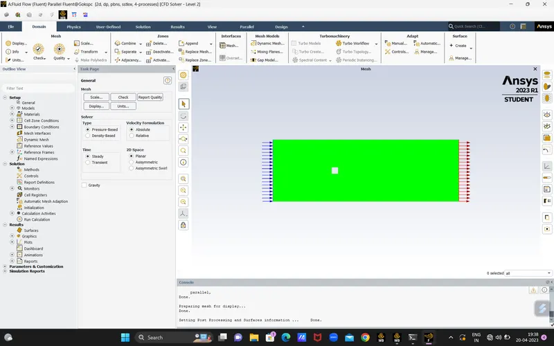
FIG 4. Steady state mesh in solver

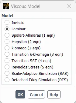
FIG 5. Selection of viscous model

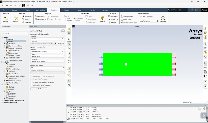
FIG 6. Changing into SIMPLE scheme

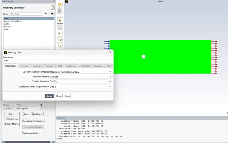
FIG 7. Entering inlet values

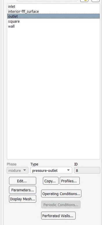
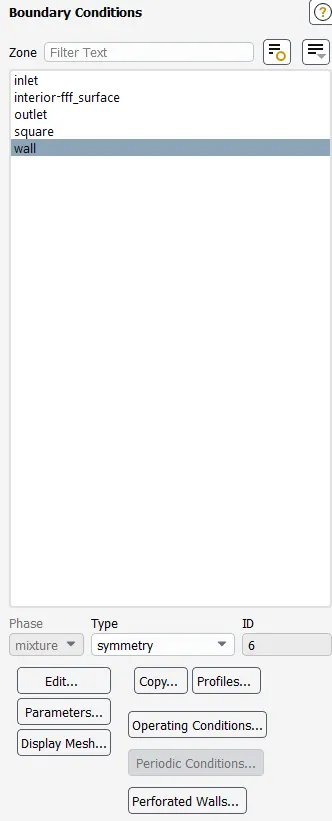
FIG 8. Applying boundary conditions

RESULTS:

Simulation of the flow over a square and explaination of the phenomenon of Karman vortex street is done.

[Case1]-Steady state:

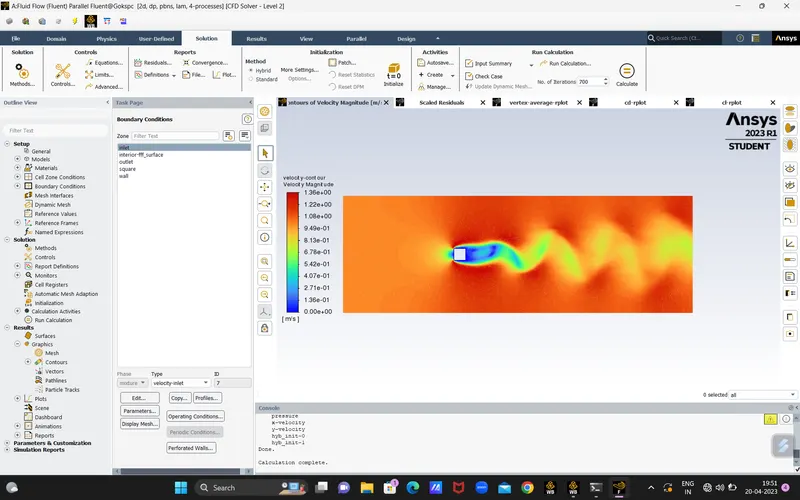
FIG 9. Velocity magnitude contour (case1)

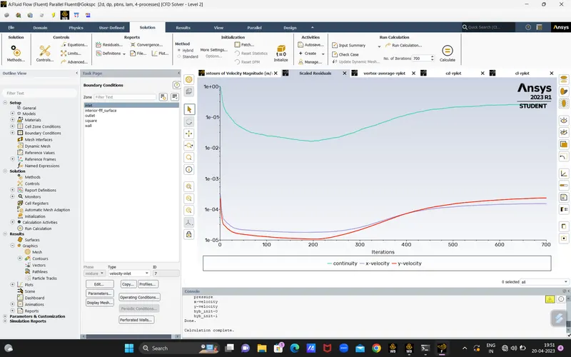
FIG 10. Residual plot(case1)

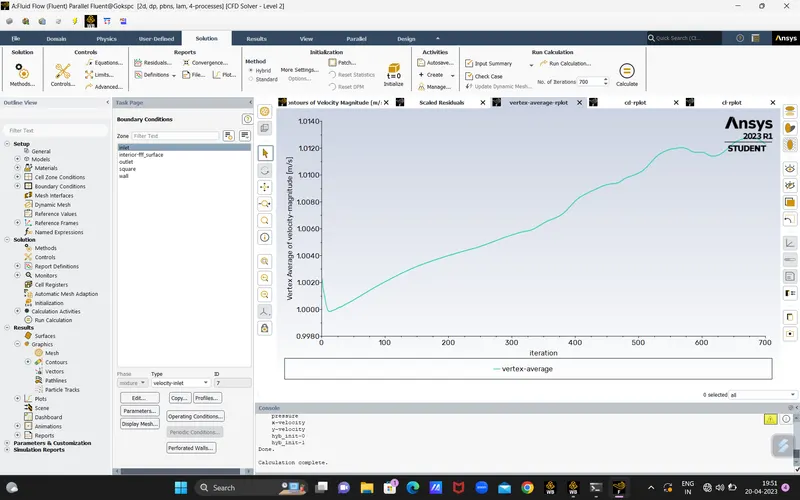
FIG 11. Vertex average plot(case1)

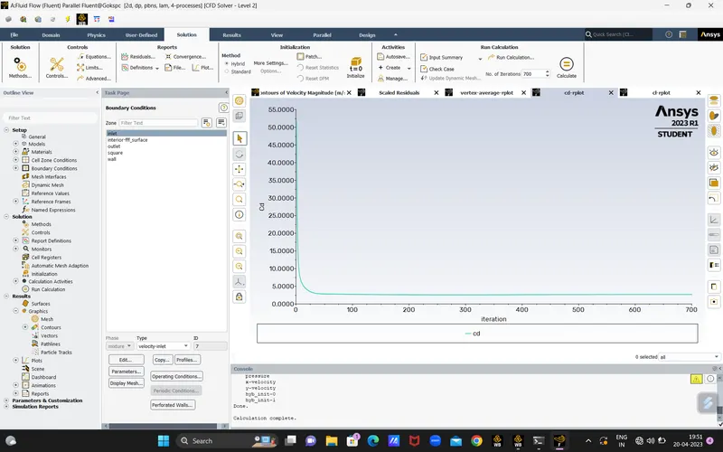
FIG 12. Coeffecient of drag plot(case1)

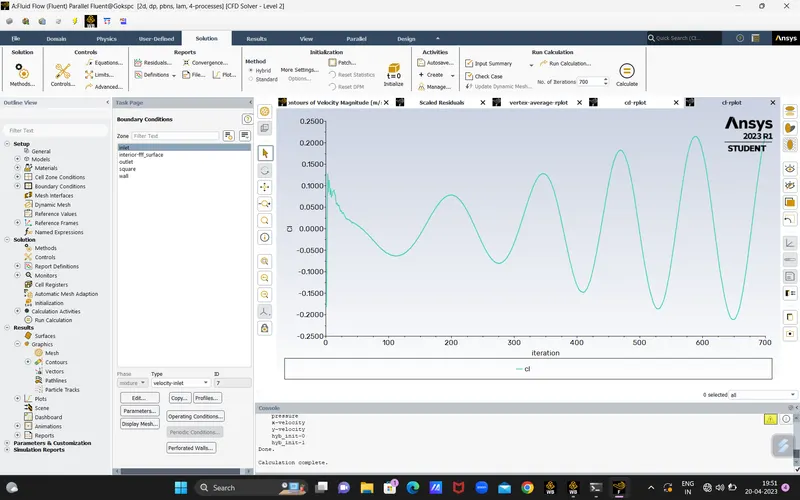
FIG 13. Coeffecient of lift plot(case1)

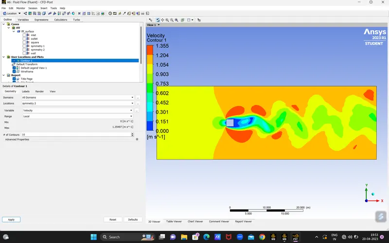
FIG 14. Velocity contour result(case1)

Case2-Unsteady state:

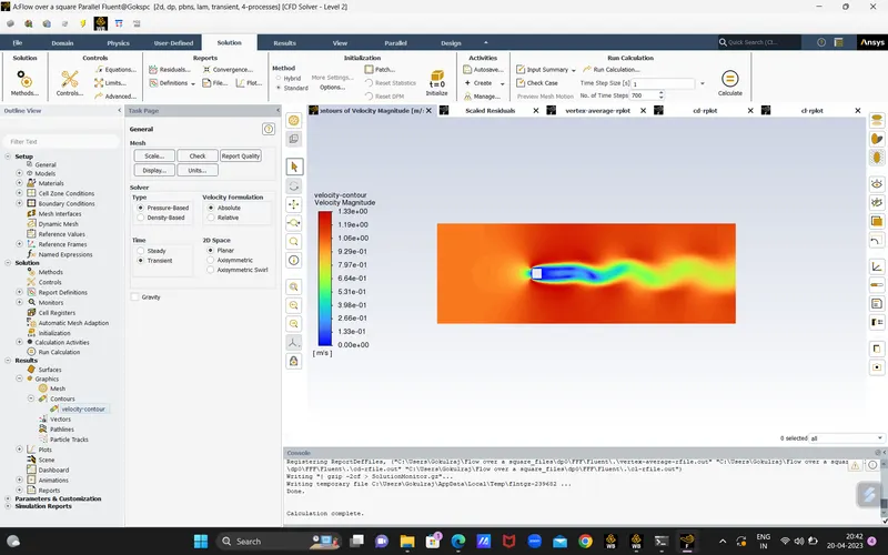
FIG 15. Velocity magnitude contour (case2)

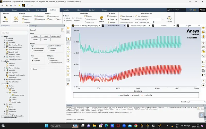
FIG 16. Residual plot(case2)

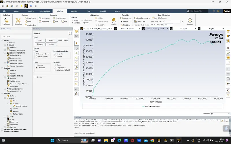
FIG 17. Vertex average plot(case2)

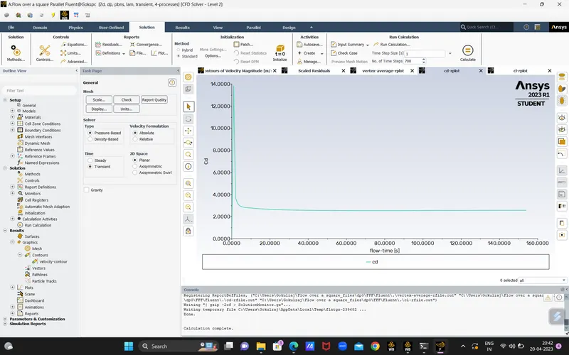
FIG 18. Coeffecient of drag plot(case2)

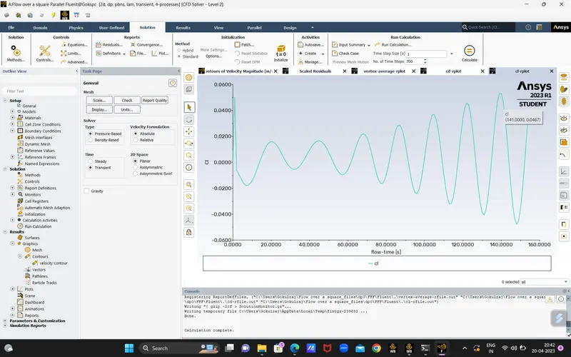
FIG 19. Coeffecient of lift plot(case2)

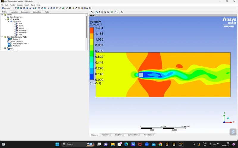
FIG 20. Velocity contour result(case2)

CONCLUSION:

S/NO.	Reynold's number(Re)	Strouhal number(S)	Velocity(m/s)
1	100	0.16	1

The velocity is calculated from the reynold's number and with that value the strouhal nuumber is calculated.

REFERENCE:

1. Strouhal number for cylinders Calculator | Calculate Strouhal number for cylinders (calculatoratoz.com)
2. Y+ Calculator | CFD Streamline
3. Reynolds Number calculator and velocity calculator for water pipes. (herramientasingenieria.com)