Week 1- Mixing Tee
AIM:
- To set up steady-state simulations to compare the mixing effectiveness when hot inlet temperature is 360C & the Cold inlet is at 190C.
case 1:
Short mixing tee with a hot inlet velocity of 3m/s.
Momentum ratio of 2, 4.
Case 2 :
Long mixing tee with a hot inlet velocity of 3m/s.
Momentum ratio of 2, 4.
2. To view the results along and across the pipe for velocity and temperature contour and line plots.
3. To compare the results in a table and discuss it in conclusion.
INTRODUCTION:
Mixing tees is an object in which two fluid streams mix are widely used in the petroleum& chemical industries. When there is a large temperature difference between two streams, large metal temperature fluctuations can occur in the region where the two streams meet if proper design steps are not taken. The temperature fluctuations in the metal can lead to thermal fatigue of the pressure boundary piping. If wall cracking occurs, the fluid may leak, possibly causing a fire and damage. Therefore, it is compulsory to ensure that the piping system can withstand the temperature fluctuations. Options can include improving the mixing of the two streams to reduce the temperature fluctuations through redesign of the piping system such that the momentum ratio of the two fluid streams is favorable to rapid mixing. This region includes the T-junction and a length of differing main pipe diameters downstream from the T-junction.
CFD simulations can provide accurate predictions of the mixing behavior including temperature and velocity ,etc,.
SOLVING & MODELLING APPROACH:
- Importing the geometry in fluent workbench on spaceclaim.
- Meshing the geometry and named selection.
- Setting up the solver .
- Intialization and calculation of the model.
- The results(contour & line plot).
PRE-PROCESSING & SOLVER SETTING:
1.Geometry:
- Open ansys fluent workbench.
- Open new spaceclaim geometry.
- Open files and import and the short mixing tee geometry.
- Go to prepare > volume extract > select face enclosure region > select the faces > Click on seed select > select any one of the inlet face > ok.
- The volume will be created and the shell can be suppressed to physics and disable the shell.
- Now the save the file as spaceclaim doc.
- Go to geometry > Replace the geometry > Opne the saved spaceclaim geometry > Update.
- Repeat the same process for long mixing tee.
2.Mesh:
- Open mesh, check the units and click on generate mesh.
- After mesh generation the mesh is not satisfying, so change the mesh type into quad & element size into 2mm.
- Now click on generate .
- Then click on the surface select and select the surfaces to create named selections such as inlet_y, inlet_y & outlet.
- Now close and update the mesh workbench.
- Repeat the same process fro long mixing tee.
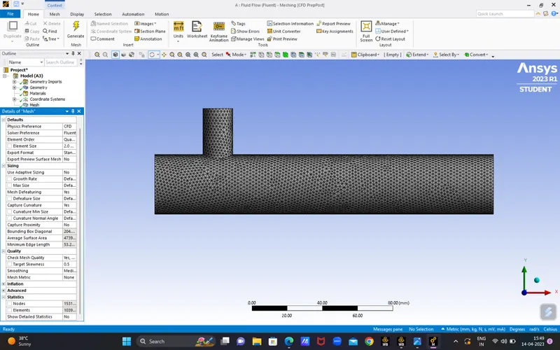
FIG 1.Mesh of case1 geometry
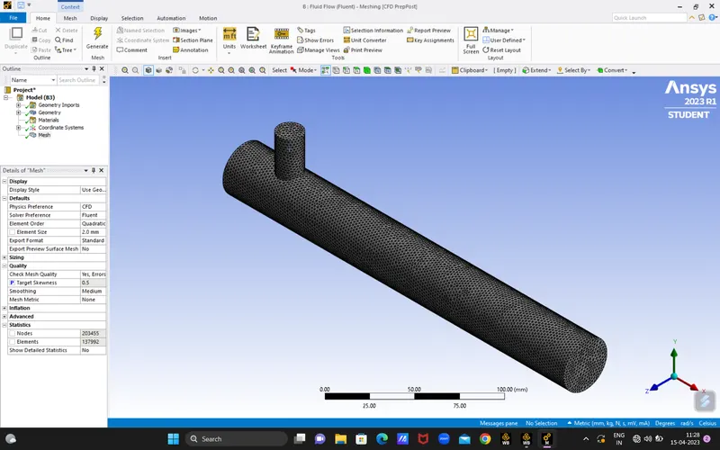
FIG 2.Mesh of case2 geometry
3.Solver setup:
(a)case-1(short mixing tee)
- Solver- steady state.
- Turn on- energy equation (since we need temperature0.
- Turbulence model- laminar( we can also use K-epsilon).
- Boundary conditions > Inlet_x(edit) > Velocity inlet > Variable-temperature > Inlet_x temperature(39degrees) > Inlet_y(19degrees) > Ok.
- Give the "inlet velocity of Inlet_x as 3m/s & Inlet_y as 6m/s".
- Go to solution > create surface report definition > Area weighted average report > Give it a title > Change field variable into - Temperature > Ok.
- Repeat the same process in solution for velocity also.
- Click on Intialize .
- Give the number of iterations as 200 and click on calculate.
- Close the solver.
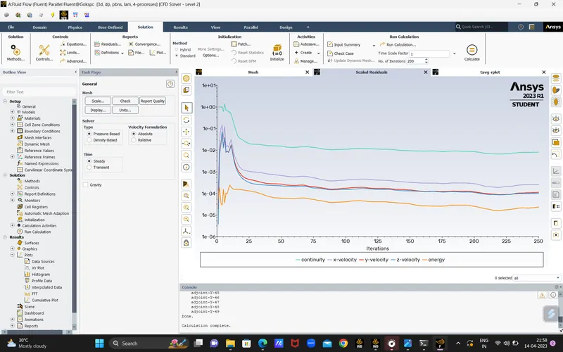
FIG 3. Residual plot for case1
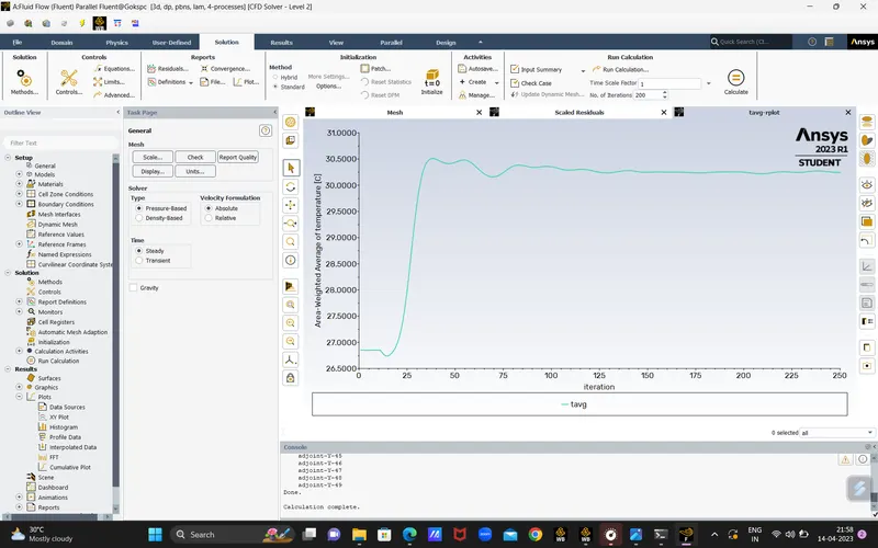
FIG 4. Tavg plot for case1
(b)case-2:
- In this case we repeat the same process as case-1, this case we use long mixing tee geometry and just changing the "velocity of Inlet_y to 12m/s".
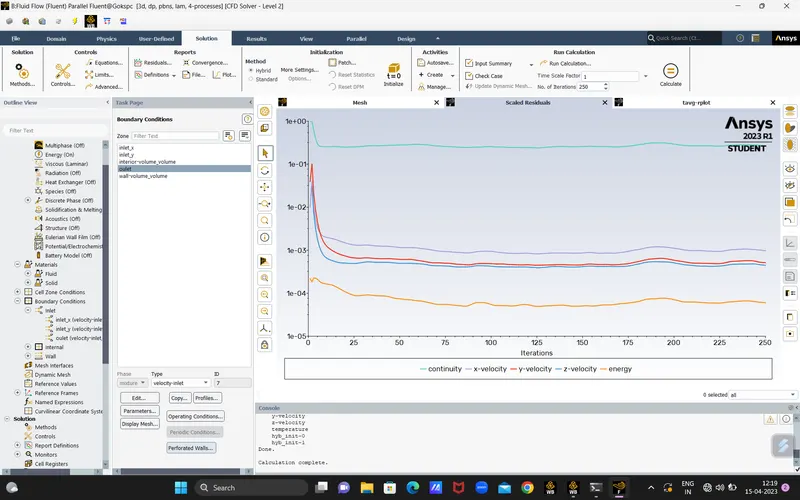
FIG 5. Residual plot for case2
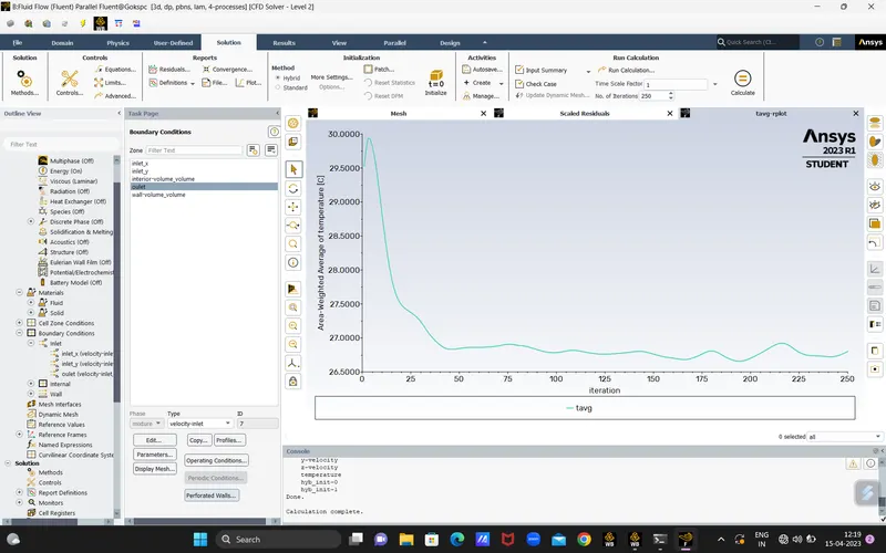
FIG 6. Tavg plot for case2
POST-PROCESSING:
1.Contours:
- Create a new contour-1 > Change into variables > Temperature > select the volume to display.
- Create contour-2 > variables > velocity > select the volume.
- Create a plane along YZ axis & Change the variables to see along and across the pipe by duplicating the plane again and moving it to another location fro many views.
- Repeat the process for both the cases.
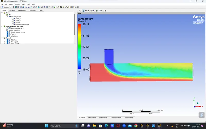
FIG 7. Temperature contour for case1
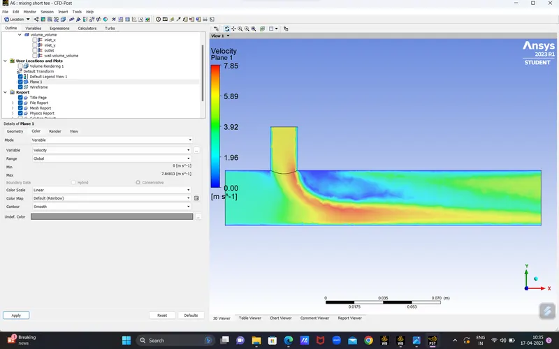
FIG 8. Velocity contour for case1
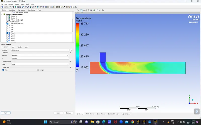
FIG 9. Temperature contour for case2
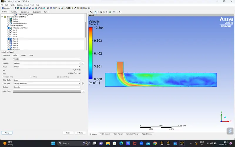
FIG 10. Velocity contour for case2
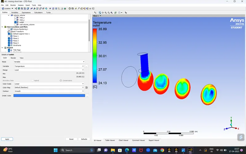
FIG 11. Temperature across case1
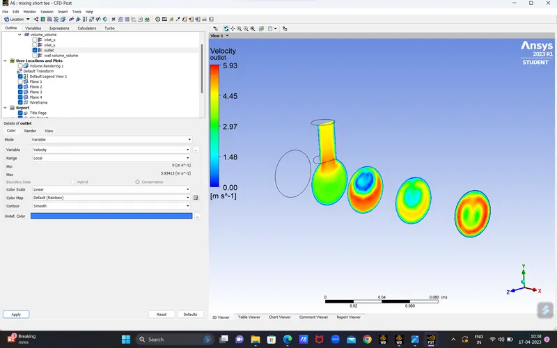
FIG 12. Velocity across case1
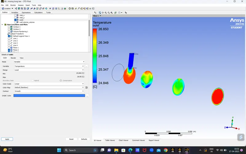
FIG 13. Temperature across case2
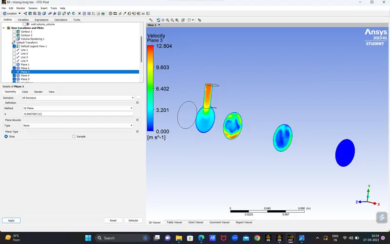
FIG 14. Velocity across case2
2.Lines:
- Create a new line-1 > Change the variables for temperature & velocity > Set the line coordinates to make it view along and across the pipe.
- Repeat the process for both the cases.
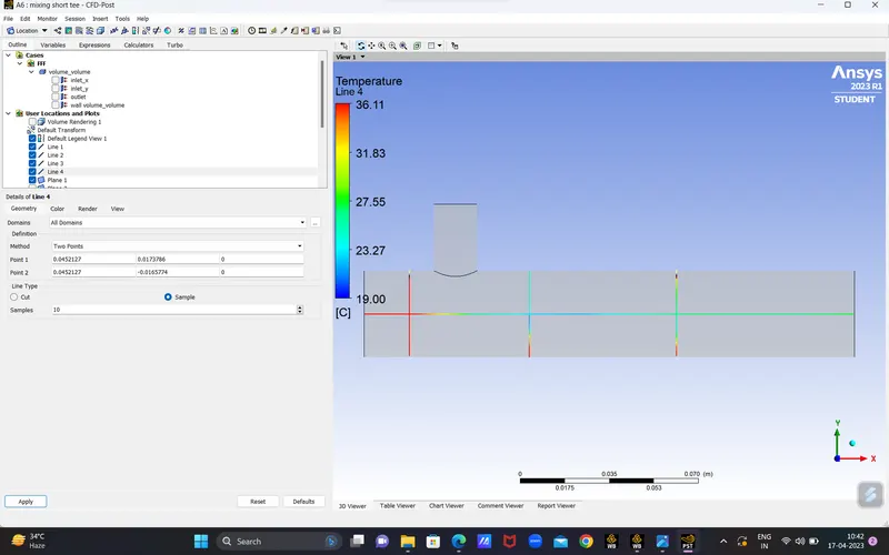
FIG 15. Temperature lines in case1
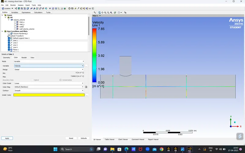
FIG 16. Velocity lines in case1
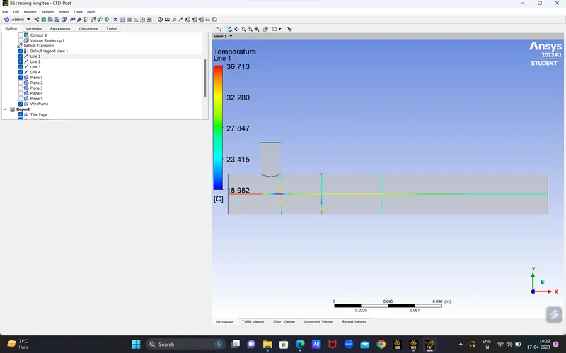
FIG 17. Temperature lines in case2
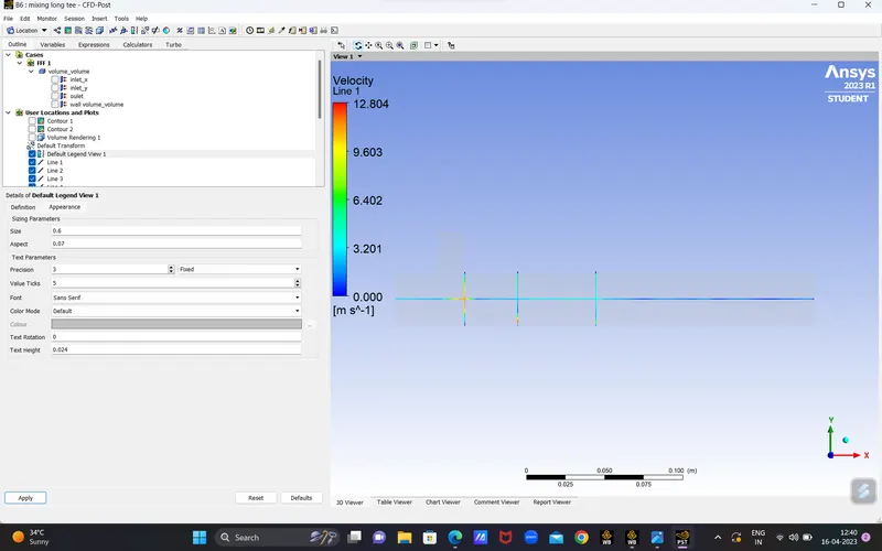
FIG 18. Velocity lines in case2
3.Charts:
- Create a new chart-1 > Input the data series > Change the variables for velocity and temperature > Setup X & Y axis > apply.
- Repeat the same process for both the cases.
- Close the results and update the project and save it.
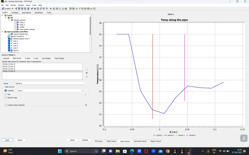
FIG 19. Temperature chart for case1
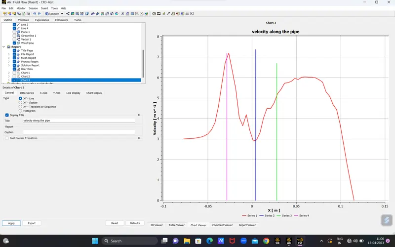
FIG 20. Velocity chart for case1
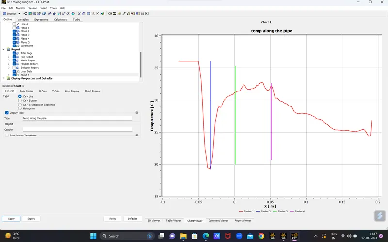
FIG 21. Temperature chart for case2
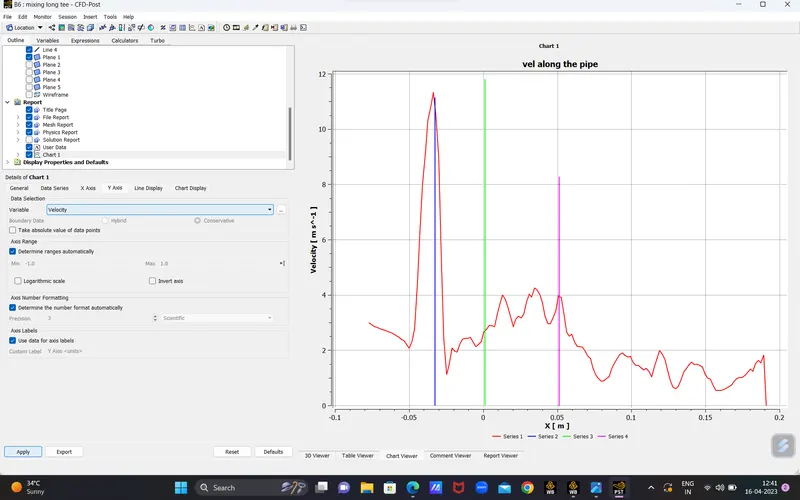
FIG 22. Velocity chart for case2
RESULTS:
The project is completed and all the objectives are met, also the results are discussed below.
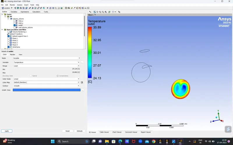
FIG 23. Temperature at outlet(case1)
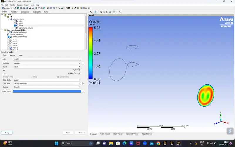
FIG 24. Velocity at outlet(case1)
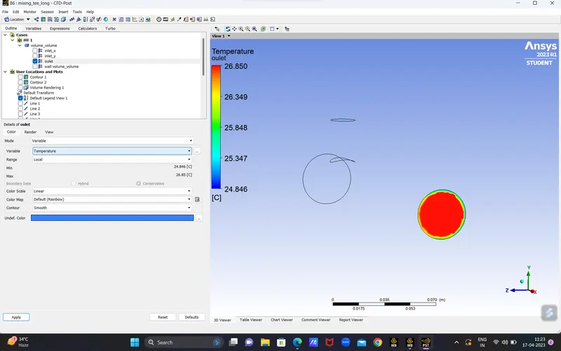
FIG 25. Temperature at outlet(case2)
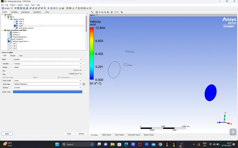
FIG 26. Velocity at outlet(case2)
CONCLUSION:
| S/NO | COMPONENTS | CASE 1 | CASE 2 |
| 1 | cell count | 103972 | 141125 |
| 2 | average outlet temperature | 33 | 31.5 |
| 3 | number of iterations for convergence | 200 | 250 |