Week 2 - Flow over a Cylinder.
AIM :
Simulate the flow over a cylinder and explain the phenomenon of Karman vortex street.
PART-I
- Simulate the flow with the steady and unsteady case and calculate the Strouhal Number for Re= 100.
PART-II
- Calculate the coefficient of drag and lift over a cylinder by setting the Reynolds number to 10,100,1000,10000 & 100000. (Run with steady solver)
- Discuss the effect of Reynolds number on the coefficient of drag. [ Results should be validated with any standard literature and error should be within 5 %]
INTRODUCTION :
1. Flow over cylinder:
In spite of extensive experimental and numerical studies of almost over a century, flow around a circular cylinder still remains a challenging problem in fluid mechanics, where intensive investigations are continued even today to understand the complex unsteady dynamics of the cylinder wake flow. Cross-flow normal to the axis of a stationary circular cylinder and the associated problems of heat and mass transport are encountered in a
wide variety of engineering applications. Both experimental measurements and numerical computations have confirmed the onset of instability of the wake flow behind a cylinder beyond a critical Reynolds number, leading finally to a kind of periodic flow identified by definite frequencies, well-known in the literature as the Von Karman vortex street. In the case of laminar flow past cylinders with regular polygonal cross-section, the flow
usually separates at one or more sharp corners of the cross-section geometry itself, forming a system of vortices in the wake on either side of the mid symmetry plane. On the other hand, for a circular cylinder, where the point of flow separation is decided by the nature of the upstream boundary layer, the physics of the flow is much more complex than what its relatively simple shape might suggest.
2. Strouhal number:
In dimensional analysis, the Strouhal number is a dimensionless number describing oscillating flow mechanisms.
The Strouhal number is often given as
St=fDU′">St= fD / U
Where,
f= frequency of vortex shedding
D= characteristic diameter of the cylinder
U'= fluid flow velocity
3. Co-efficient of drag:
In fluid dynamics, the drag coefficient (cd)">(cd)(cd) is a dimensionless quantity that is used to quantify the drag or resistance of an object in a fluid environment, such as air or water. It is used in the drag equation in which a lower drag coefficient indicates the object will have a less aerodynamic or hydrodynamic drag. The drag coefficient is always associated with a particular surface area.
The drag coefficient cd">cdcd is defined as
Cd=2⋅Fdρu2A">Cd= 2 ⋅ Fd / ρu^2 A
4. Co-efficient of lift:
The lift coefficient (CL">CLCL) is a dimensionless coefficient that relates the lift generated by a lifting body to the fluid density around the body, the fluid velocity, and an associated reference area. A lifting body is a foil or a complete foil-bearing body such as a fixed-wing aircraft. CL is a function of the angle of the body to the flow, its Reynolds number, and its Mach number. The section lift coefficient cl refers to the dynamic lift characteristics of a two-dimensional foil section, with the reference area replaced by the foil chord.
CL≡LqS=L12ρu2S=2Lρu2S">CL ≡ L / qS= L / 0.5ρu^2 S= 2L/ρu^2
where
L is the lift force,
S is the relevant surface area and
q is the fluid dynamic pressure, in turn, linked to the fluid density, and to the flow speed.
5. Phenomenon of Karman vortex street:
Flow over a cylinder is important in many industrial application like cooling of iron or cylindrical pipe,Circular pipes have more application in heat exchanger. High temperature flue gases flow over a circular cylinder in a cross flow.Depending on flow rate, fluid properties and size of cylinder, the flow can be laminar, transition and turbulent
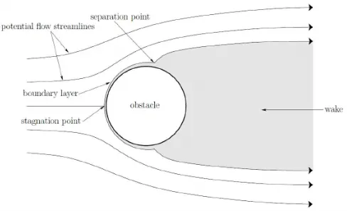
6. Karman vortex street with different reynolds number :
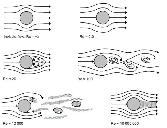
PART 1 :
SOLVING AND MODELLING APPROACH OF STEADY AND UNSTEADY FLOW :
GEOMETRY -
CHANGE UNITS FROM FILES OPTION AND SPACECLAIM OPTIONS INTO METERS
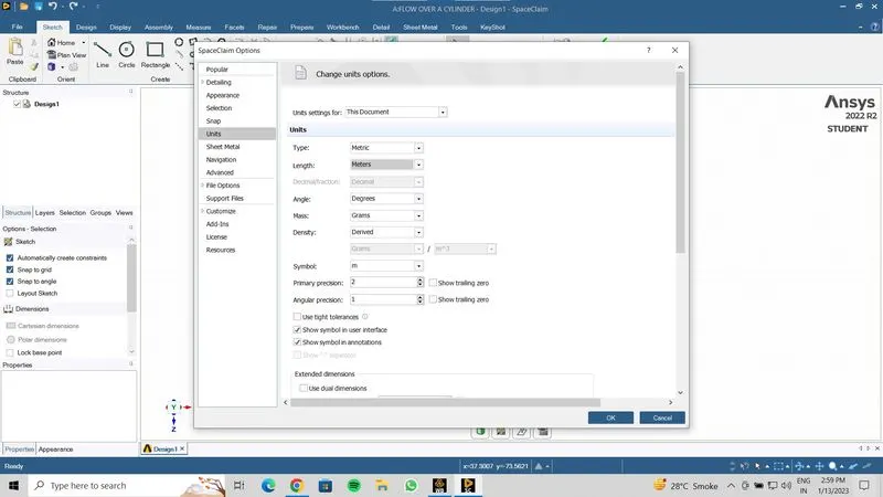
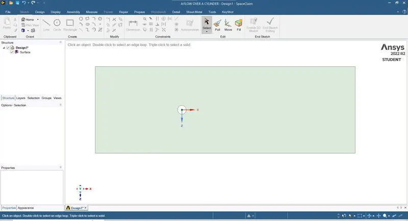
OPEN SPACECLAIM AND DRAW THE 2D GEOMETRY.
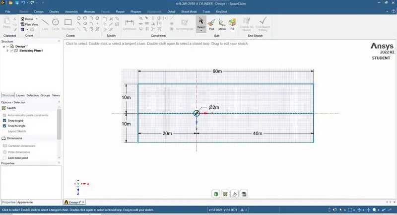
THE 2D GEOMETRY IS CREATED BY USING THE ABOVE DIMENSION THEN THE INSIDE CYLINDER IS DELETED IN ORDER TO CARRY OUT THE SIMULATION. BY USING PULL TOOL AND SELECT.
MESH :
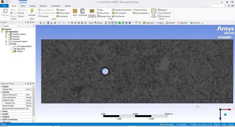
BY DEFAULT ANSYS CREATES THE QUADRILATERAL MESH OF DEFAULT SIZE. WE NEED TO CONVERT IT TO TRIANGLES.USE ELEMENT SIZE 0.25M
TO CHANGE THE MESHING METHOD. GO TO MESH => INSERT => METHOD => SELECT FACE => METHOD (TRIANGLES) => GENERATE MESH
TO AVOID INACCURACY IN THE SOLUTION THE SHARP CORNERS AROUND THE CIRCLE ARE CONVERTED INTO LARGE NUMBER OF EDGES.
TO DO THAT GO TO MESH => INSERT => SIZING => SELECT EDGE => TYPE (NUMBER OF DIVISIONS) => ENTER 36 AND GENERATE MESH
SINCE THE FLOW AROUND THE CYLINDER IS IMPORTANT, THE INFLATION LAYER IS CREATED AROUND THE CYLINDER
TO CREATE A INFLATION LAYER GO TO MESH => INSERT => INFLATION => SELECT FACE => SELECT EDGE => NUMBER OF LAYERS => ENTER NUMBER AND GENERATE MESH
FLUENT SETUP:
UPDATE THE MESH AND SOLUTION ALWAYS.
|
SETUP |
STEADY-STATE |
UNSTEADY STATE |
|
SOLVER TYPE |
Pressure based |
Pressure based |
|
VELOCITY FORMULATION |
Absolute |
Absolute |
|
TIME |
Steady |
Transient |
|
VISCOUS MODEL |
Laminar |
Laminar |
|
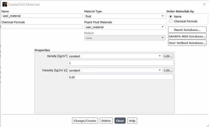
MATERIAL |
User material |
User material |
|
CELL ZONES |
Fluid type: user material Density – 1 kg/m3 Dynamic viscosity – 0.02 kg/ms |
Fluid type: user material Density – 1 kg/m3 Dynamic viscosity – 0.02 kg/ms |
|
BOUNDARIES |
Velocity magnitude 1m/s
Gauge pressure – 0 pa
Condition - No slip |
Velocity magnitude 1m/s
Gauge pressure – 0 pa
Condition - No slip |
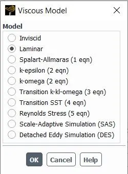
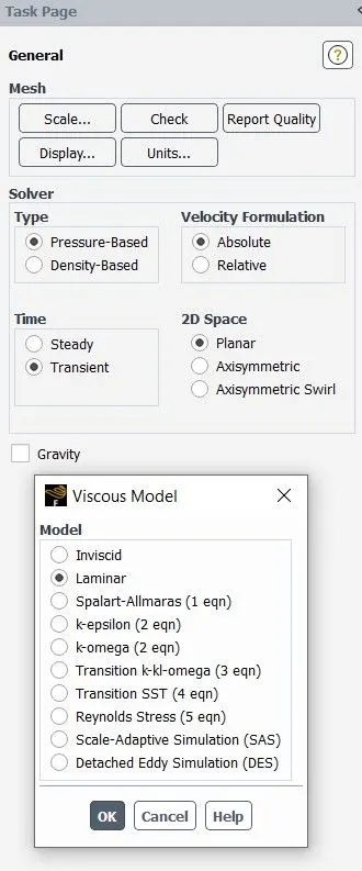
SELECT THE FLUENT SETUP AS GIVEN IN ABOVE TABLE.
CREATE A VERTEX AVERAGE OF VELOCITY MAGNITUDE USING SURFACE REPORT AT A MONITOR POINT 8M AWAY FROM THE CENTER OF THE CYLINDER TO THE RIGHT OF THE CYLINDER ALONG X-DIRECTION.
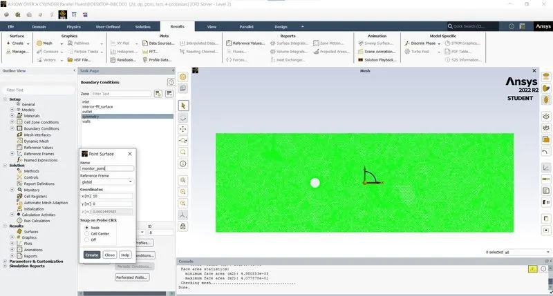
TO READ A AVERAGE VELOCITY VALUE AT ABOVE `ONITOR POINT GO TO
DEFINATIONS - SURFACE REPORT - VERTEX AVERAGE.
COEFFICIENT OF DRAG AND COEFFICIENT OF LIFT REPORT CREATED USING FORCE REPORT.
FOR DRAG GO TO DEFINATIONS - NEW - FORCE REPORT - DRAG
FOR LIFT GO TO DEFINATIONS - NEW - FORCE REPORT - LIFT
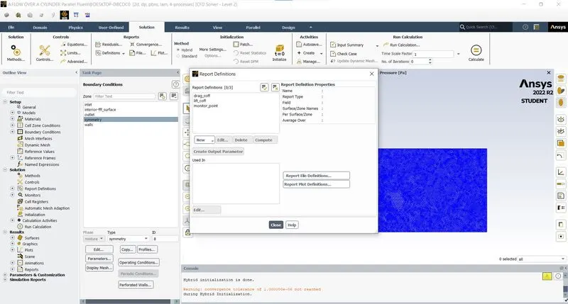
INITIALIZATION: Hybrid for steady state
The standard for unsteady state
ACTIVITIES: Contour plots of pressure and velocity and solution animation are created after initialize the solution.
For steady-state – No of iterations= 500
For transient state – Time step = 0.1
No of iterations = 500
RESULTS :
STEADY STATE-
RESIDUAL -
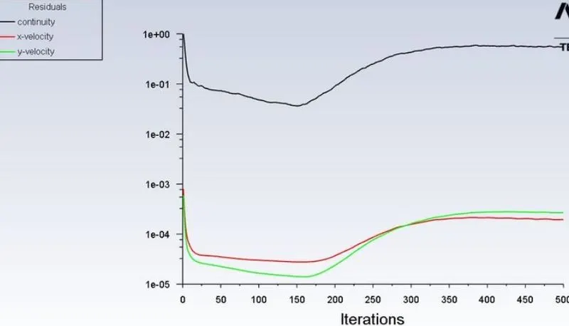
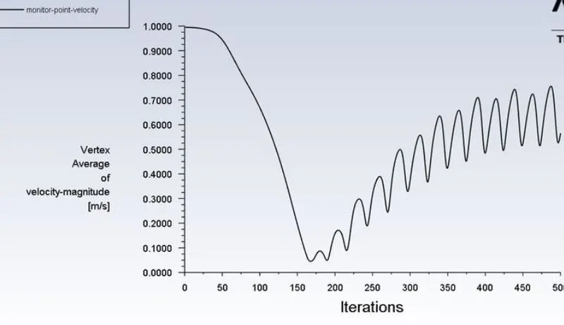
MONITOR POINT FUNCTION -
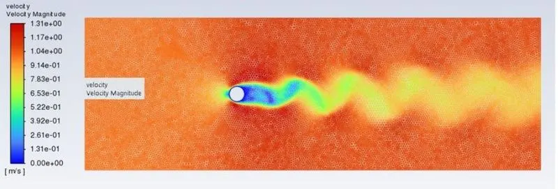
VELOCITY CONTOUR -
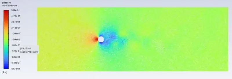
PRESSURE CONTOUR -
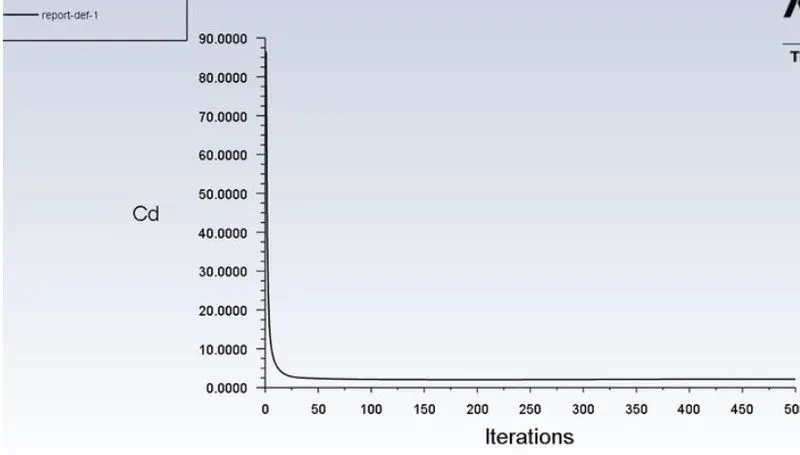
DRAG PLOT -
LIFT PLOT -
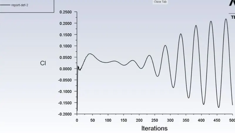
The strohaul number cannot be calculated for the steady state as we don't calculate the flow with respect to time.
TRANSIENT :
RESIDUAL -
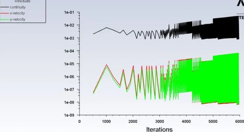
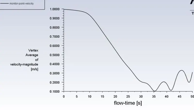
MONITOR POINT FUNCTION -
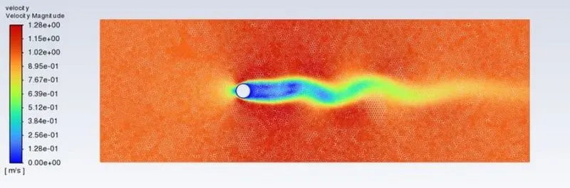
VELOCITY CONTOUR -
PRESSURE CONTOUR -
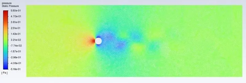
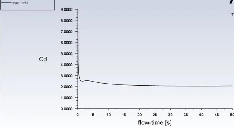
DRAG PLOT -
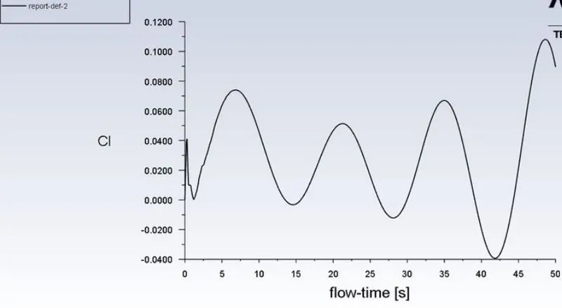
LIFT PLOT -
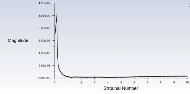
STROHAUL NUMBER -
SUMMARY :
Strohaul number = 0.01.
| CASES | REYNOLDS NUMBER | INLET VELOCITY | Cd | Cl | MONITOR VELOCITY |
| STEADY STATE | 100 | 1m/s | 1.367848 | 0.17997243 | 0.62m/s |
| TRANSIENT STATE | 100 | 1m/s | 1.2657366 | 0.018048622 | 0.27m/s |
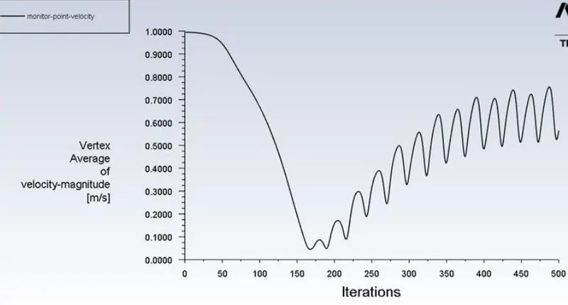
From the above cases, we can say that in the transient case the velocity starts oscillating for the monitoring point after certain iterations and the velocity at the monitoring point is greater in the case of the steady-state case as compared to the transient case.
PART 2 :
1) Simulate the flow with the steady state for Re= 10.
U = 0.1 M/S
RESIDUALS -
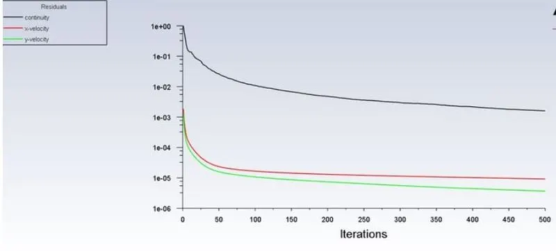
MONITOR POINT VELOCITY -
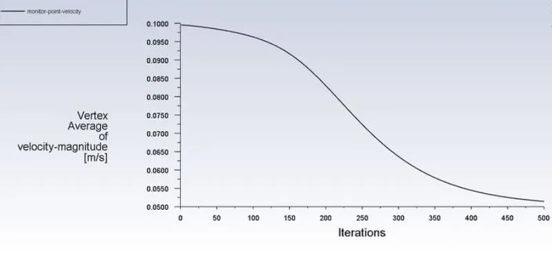
VELOCITY CONTOUR -
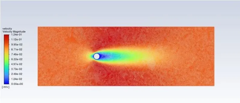
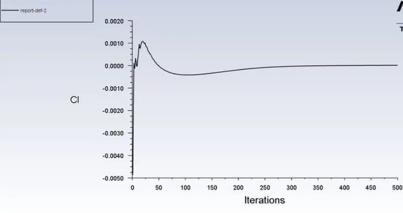
DRAG PLOT -
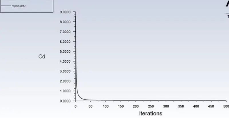
LIFT PLOT -
2) SIMULATION OF FLOW FOR THE STEADY STATE FOR Re = 100
U=1m/s
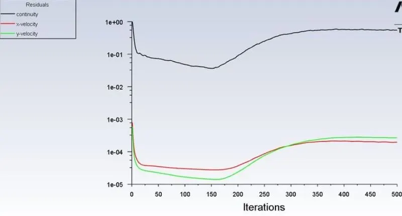
RESIDUALS -
MONITOR POINT VELOCITY -
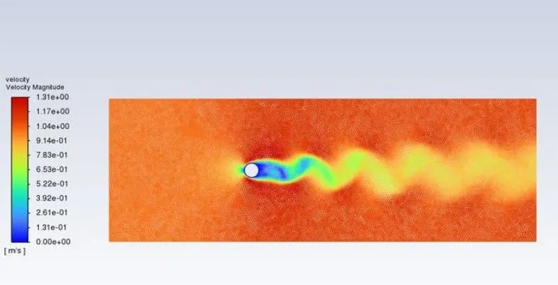
VELOCITY CONTOUR -
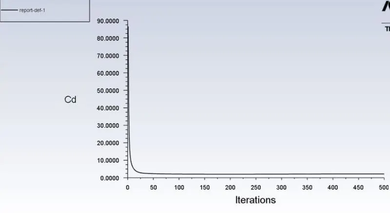
DRAG PLOT -
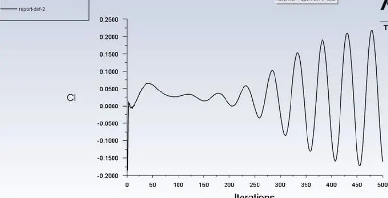
LIFT PLOT -
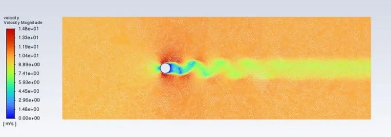
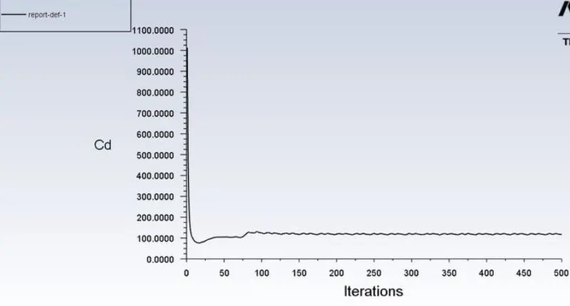
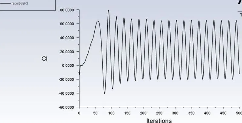
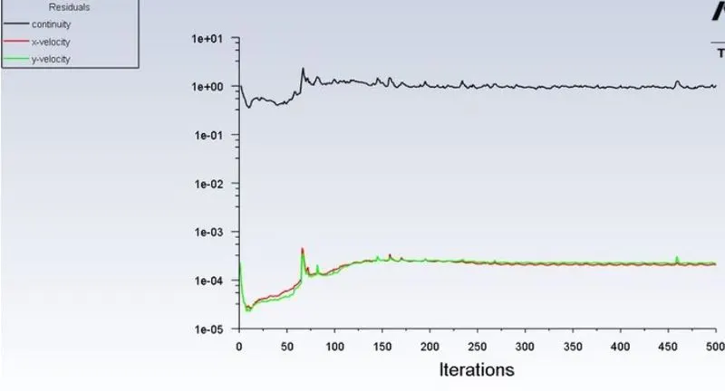
3) SIMULATION OF FLOW FOR THE STEADY STATE FOR Re = 1000
U=10m/s
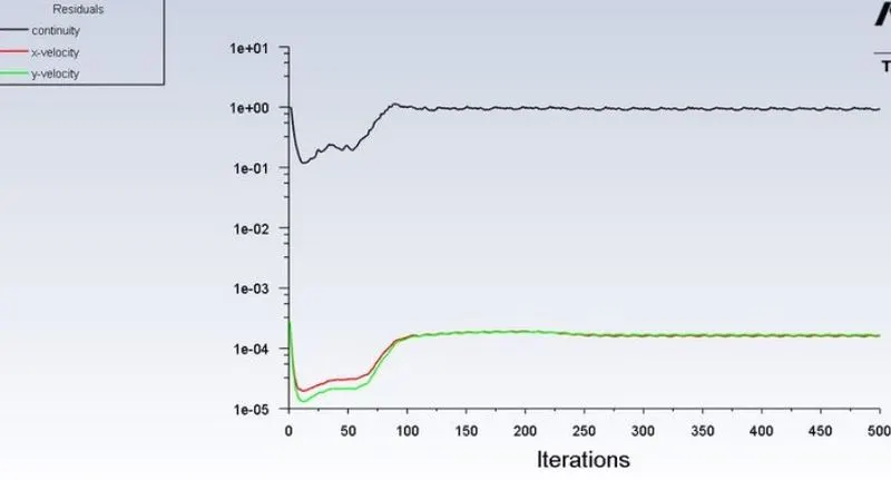
RESIDUALS -
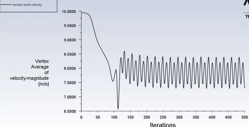
MONITOR POINT VELOCITY -
VELOCITY CONTOUR -
DRAG PLOT -
LIFT PLOT -
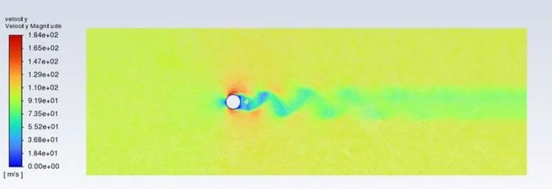
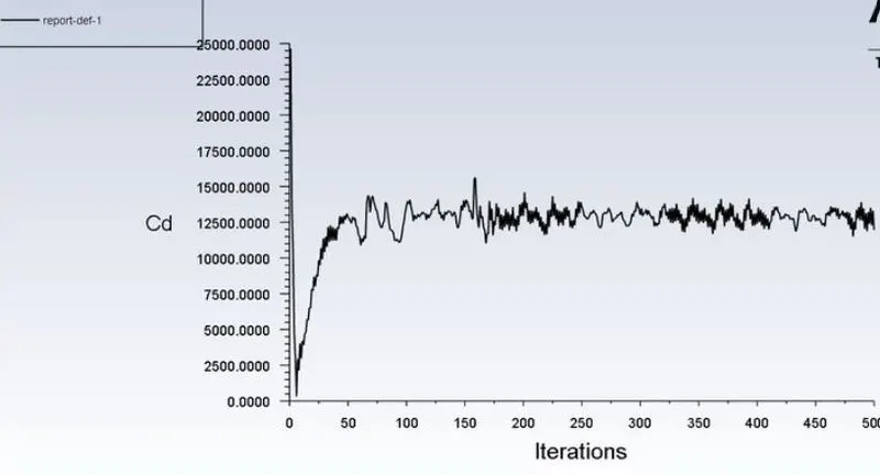
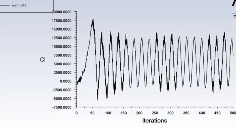
4) SIMULATION OF FLOW FOR THE STEADY STATE FOR Re = 10000
U=100m/s
RESIDUALS -
MONITOR POINT VELOCITY -
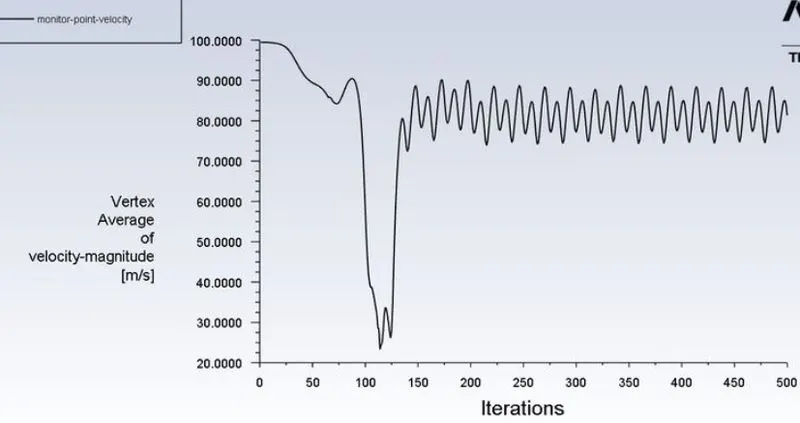
VELOCITY CONTOUR -
DRAG PLOT -
LIFT PLOT -
5) SIMULATION OF FLOW FOR THE STEADY STATE FOR Re = 100000
U=1000m/s
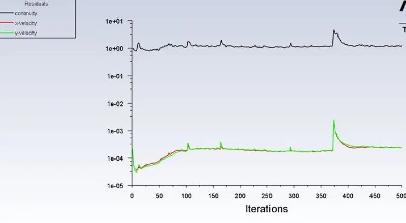
RESIDUALS -
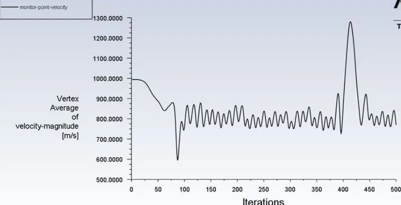
MONITOR POINT VELOCITY -
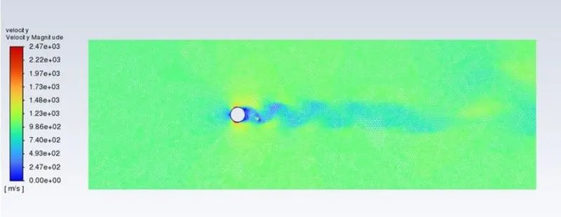
VELOCITY CONTOUR -
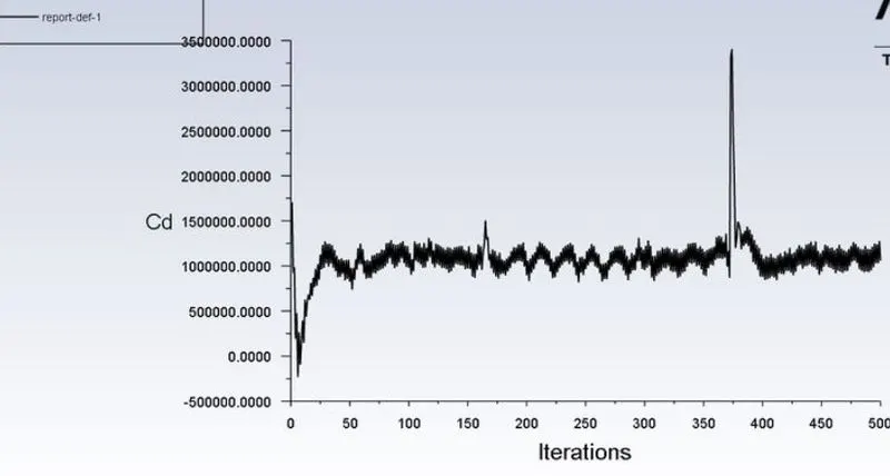
DRAG PLOT -
LIFT PLOT -
SUMMARY:
| SIMULATION | REYNOLDS NUMBER | Cd | Cl |
| 1 | 10 | 3.3314425 | -0.00085925251 |
| 2 | 100 | 1.367848 | 0.17997243 |
| 3 | 1000 | 0.86912317 | -0.331299 |
| 4 | 10000 | 0.81047329 | 0.9461438 |
| 5 | 100000 | 0.74380507 | 0.43716453 |
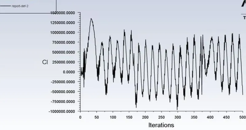
From the above plot, we can say that the value of the lift coefficient keeps on increasing as we keep increasing the velocity and Reynolds number. The drag coefficient is maximum for the lowest Reynolds number and goes on decreasing.
CONCLUSION:
- When fluid flows over the cylinder, the wake region is formed next to the cylinder due to a decrease in pressure, and recirculation of flow occurs hence flow separation occurs.
- As flow over a cylinder is transient we are unable to observe flow separation at a low Reynolds number
- As the Reynolds number increases the coefficient of drag decreases.
- Strauhal number for an unsteady state with Reynolds number 100 is 0.01.
(FAIZ AMIR AZMI)