Simulation of flow over the cylinder and observing the Karman Vortex phenomenon
Aim: Simulation of flow over the cylinder and observing the Karman Vortex phenomenon
Objective:
- Prepare the computational domain for the given problem of an external fluid flow simulation
- Understand the formation of vortices around a bluff body, deduce the drag and lift coefficient and study the effect of Reynolds number on the vortices so formed
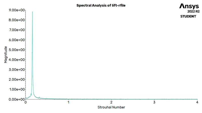
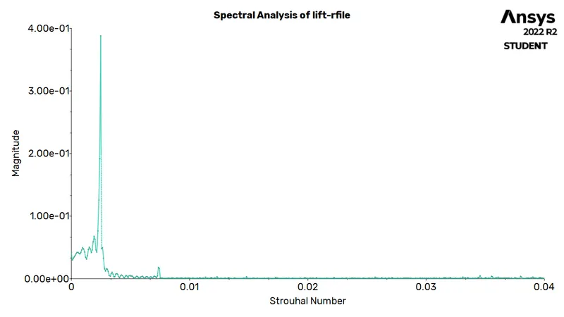
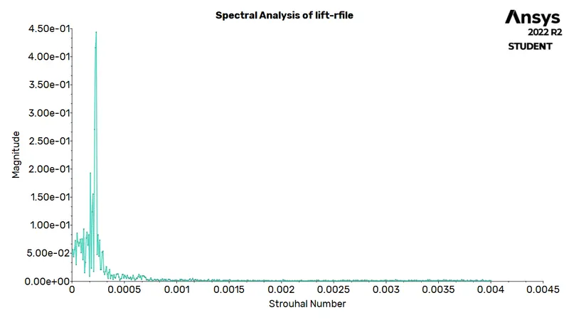
- Understand the principle of Karman vortex street and evaluate Strouhal number for the given flow over the cylinder
Introduction:
In fluid mechanics, external flows are defined by the relative motion between the fluid and a body which is completely immersed in the fluid and thereby, boundary layers develop freely (unconfined). The flow fields and geometries for most external flows is quite complicated to be studied analytically and hence co-relations are developed for studying the flow characteristics.
Since, the body is immersed in a fluid, it experiences resistance in the relative motion occuring between them. Drag force acting on an object opposes the motion of the object. For a frame of reference moving with the object, this force acts in the direction of the flow. There are some components of drag force; friction drag (results by integrating shear stress in the direction of flow), induced drag (it is induced by lift and associated with the vortices forming around the object's tip), pressure (or form) drag (results from integrated surface pressure in the direction of flow). When, this drag force is non-dimensionalised by the dyanmic pressure of the free stream times the frontal area, the resulting non-dimensional number is known as drag coefficient. The net aerodynamic force on an object acting perpendicular to the motion of the object is called lift force. Non-dimensionalising this similar to drag force gives us the lift coefficient.
Bluff bodies have wakes resulting from massive flow separation over the rear body, which is a friction-dominated region formed by the surface boundary layer swept to the rear by the free stream velocity. At high Reynolds number, vortex are formed, which are structures formed in a fluid flow with concentration of vorticity (flow rotation). The alternating unsteady pattern of vortices commonly observed behind the circular cylinders is called the Karman vortex street.
Strouhal number is a dimensionless number that represents the ratio of inertial forces due to local acceleration to the inertia forces due to convective acceleration.
`St = (f L)/(U)`
where
`St ->` Strouhal Number
`f ->` shedding frequency
`L ->` characteristic length
`U ->` flow velocity
Workflow:
- Preparing the geometry
- Generate mesh for the geometry
- Setting up the solver
- Setting up the solution monitors
- Post-processing to observe the results
Ansys Fluent:
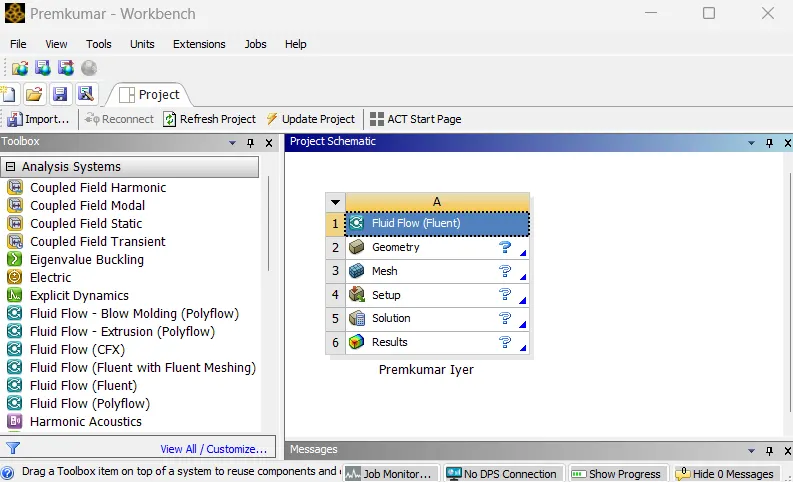 |
In the Ansys workbench project window, Fluid Flow (Fluent) is dropped into the workspace.
Preparing the geometry:
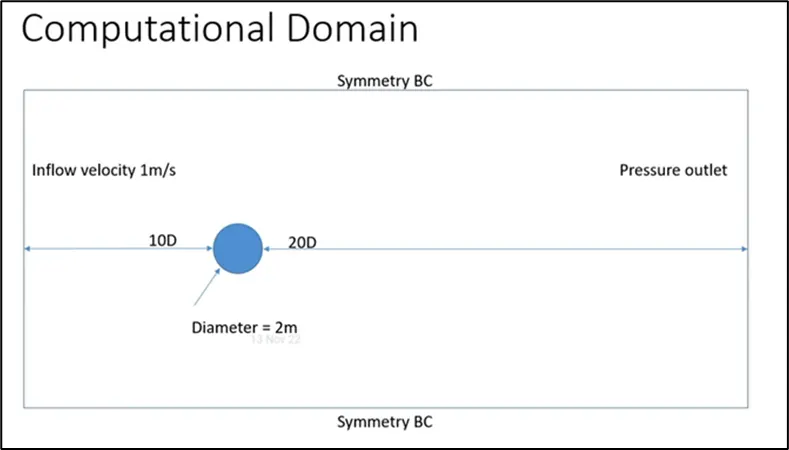
The computational domain, followed for the simulation is as shown below:
 |
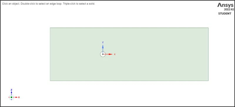 |
The computational domain, as shown before, is recreated in SpaceClaim as a 2D structure.
Generating mesh:
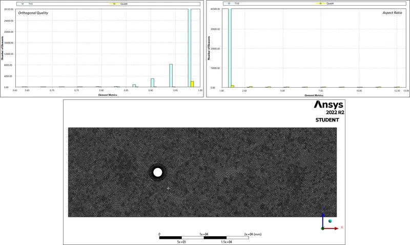
Meshing is the process, wherein the geometry is divided into smaller parts which are known as elements, so that the iterative solver can solve the governing equations across the domain. In the meshing utility, a mesh of element size 250mm is provided. Further, the method of meshing is inserted as "all traingles". Since, the cylinder body lost its curvature (or roundedness), and therefore edge sizing with 100 no.of divisions were provided. Since, the eddies are formed due to detachment from the cylinder wall, the changes happening over the cylinder walls must be effectively captured. For this, an inflation with 20 layers is provided and the first layer thickness being 5mm, which is decided based on the y+ value. Care has been taken for the volume transition to remain smooth and thus, we have the following mesh metrics:
 |
For implementing the boundary conditions, the "boundaries" must be clearly defined. To do so, the mesh utility itself has a tool; named selections. By selecting the respective faces and surfaces, the velocity inlet, the pressure outlet, symmetry and the cylinder wall as well was defined.
Seting up the solver:
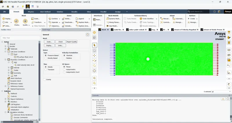 |
An important part of a CFD simulation, the setup for solver is done to obtain the solution. Firstly, the units of important parameters are set to desired units (preferably SI units). In the models tab, in the viscous models, laminar is chosen. The fluid zone contains a user defined fluid with the following properties:
| Density | : `1 Kg//m^3` |
| Viscosity | : `0.05 Pa-s` |
The only boundary condition that we need to provide is the inlet velocity (which is varied based on the Reynolds number), rest everything is left untouched. The reference values are altered with respect to the inlet.
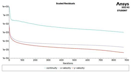
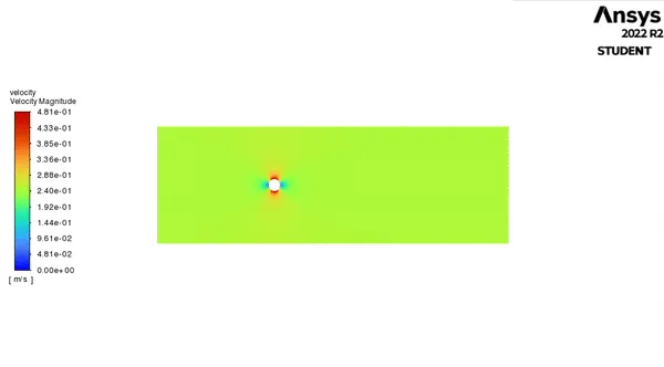
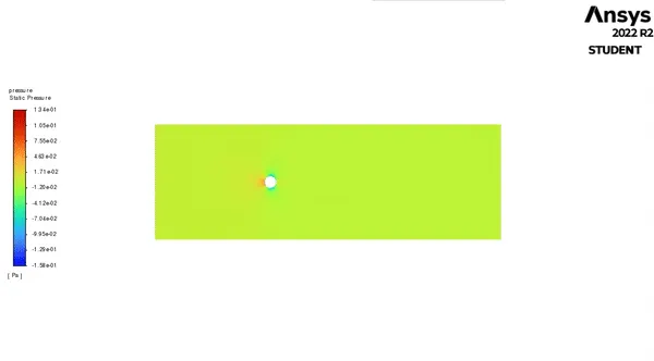
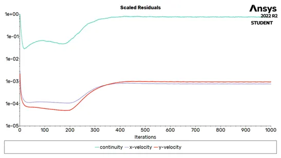
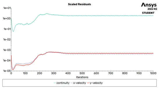
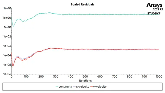
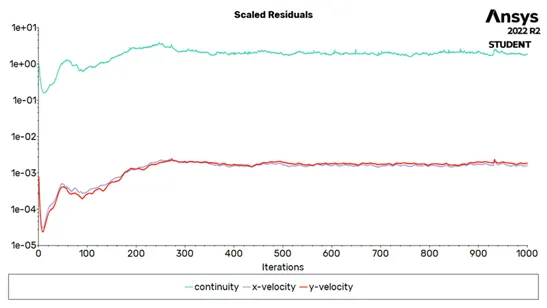
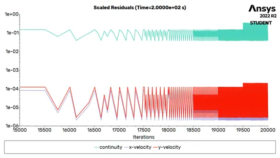
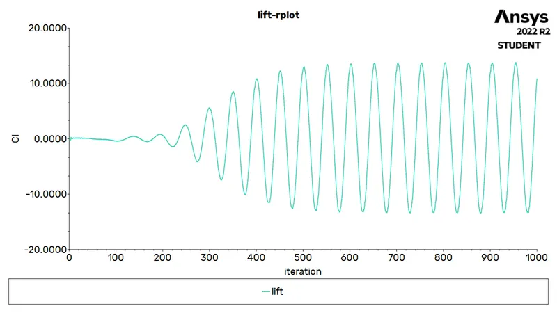
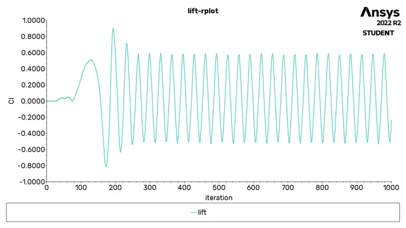
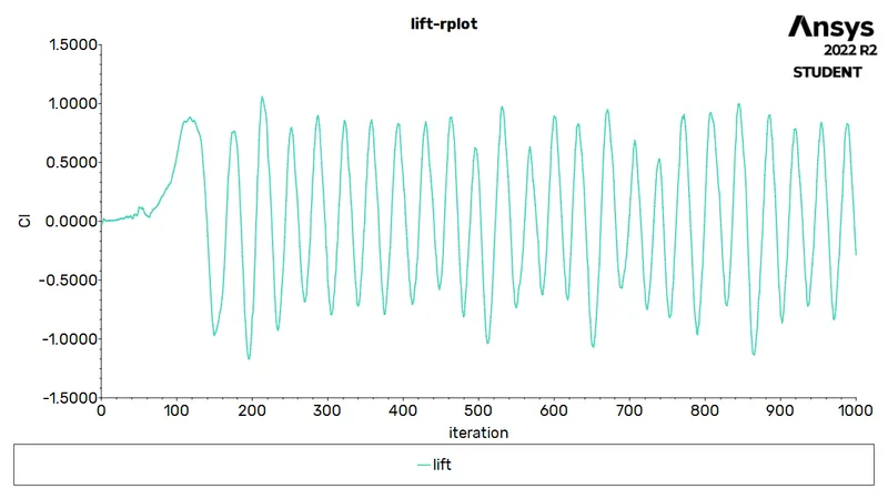
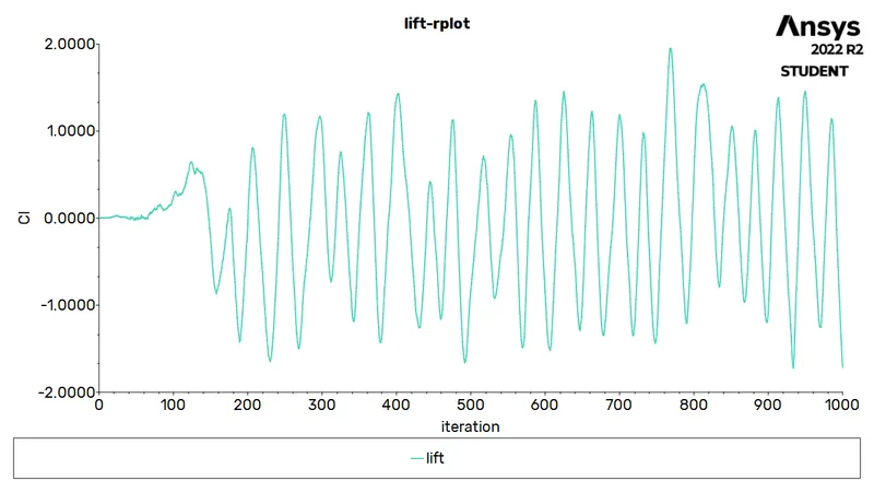
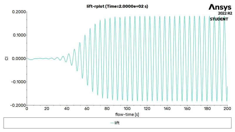
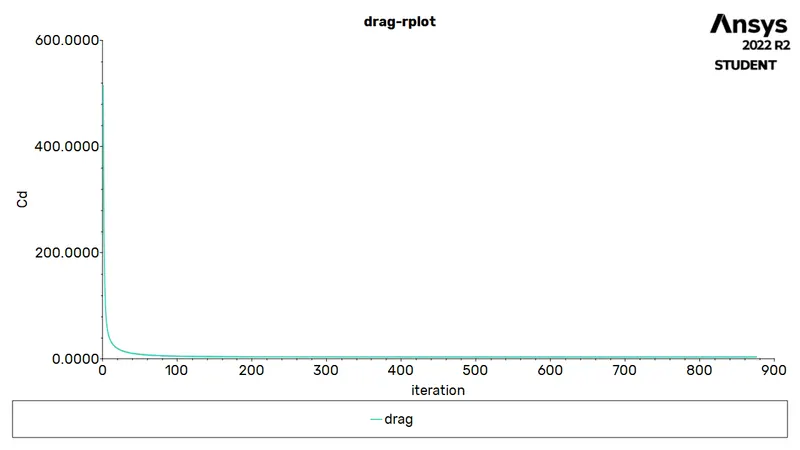
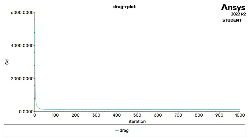
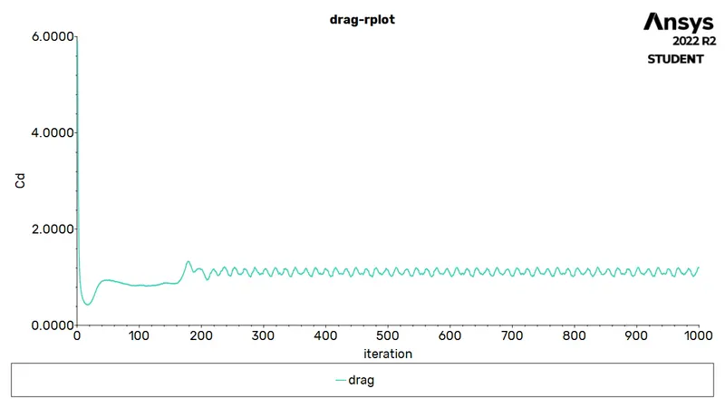
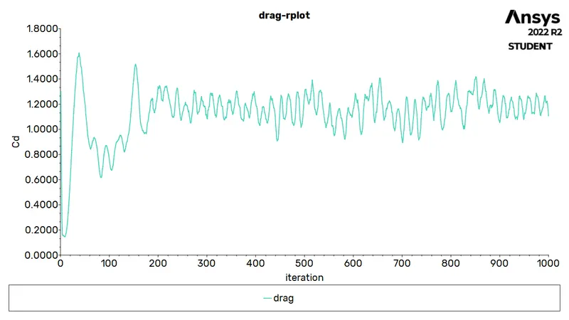
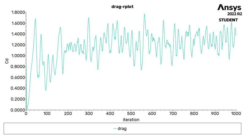
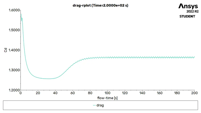
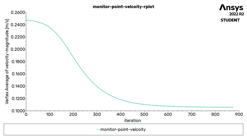
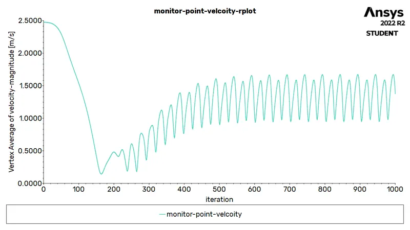
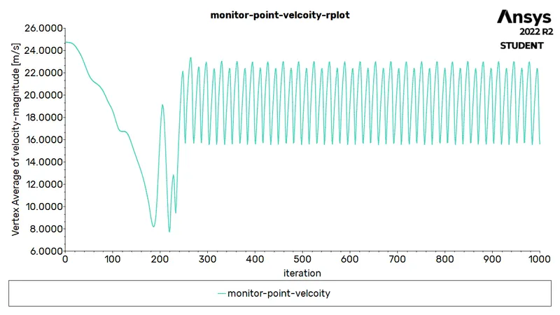
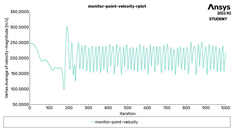
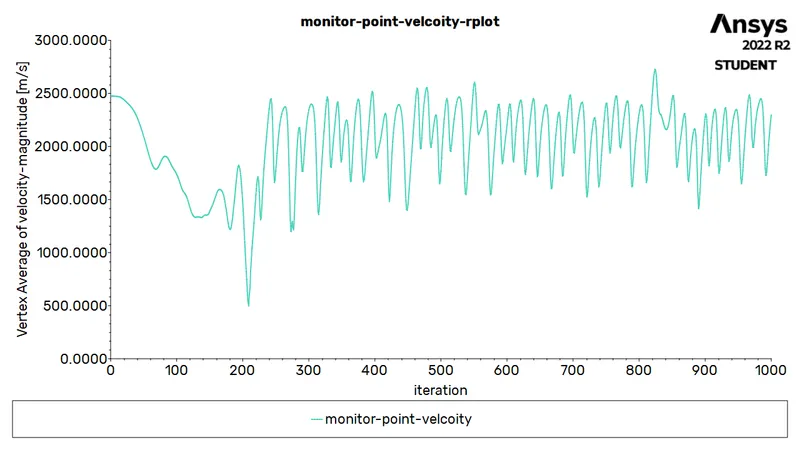
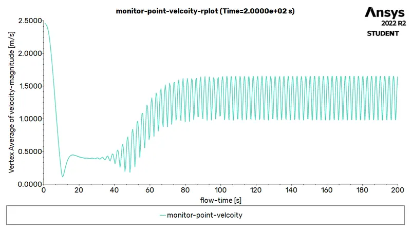
The pressure-velocity coupling is set to SIMPLE and the momentum and pressure are set to second order discretisation. A monitor point is created to capture the velocity changes behind the cylinder (in the wake region). And thus, report definitions are set to capture this velocity and the coefficient of drag and lift over the cylinder surface. The corresponding plots along with the residual plots are saved. Solution animation is generated for the velocity and pressure contours. Hybrid initialization is used to initiate the problem, thereafter, 1000 iterations (for steady) and 0.1s time step with time steps (for unsteady) are provided. After completion of the iterative procedure, FFT (fast fourier transform) is applied to determine the strouhal number.
Post-processing (Results):
|
Case |
Residual |
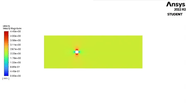
Velocity |
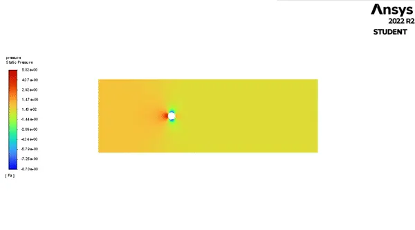
Pressure |
|
`Re 10` |
 |
 |
 |
|
`Re 100` |
 |
 |
 |
|
`Re 10^3` |
 |
 |
 |
|
`Re 10^4` |
 |
 |
 |
|
`Re 10^5` |
 |
 |
 |
|
`Re 100` |
 |
 |
 |
|
Case |
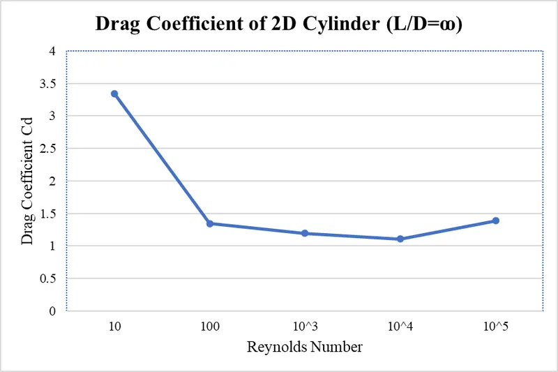
Drag |
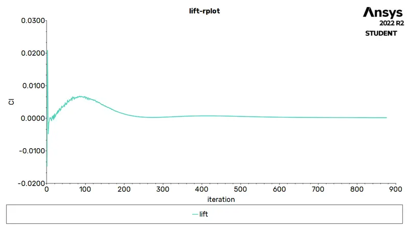
Lift Coefficient |
|
`Re 10` |
3.338571 |
 |
|
`Re 100` |
1.345938 |
 |
|
`Re 10^3` |
1.194297
|
 |
|
`Re 10^4` |
1.107112
|
 |
|
`Re 10^5` |
1.387243
|
 |
|
`Re 100` |
1.365531
|
 |
|
Case |
Monitor point |
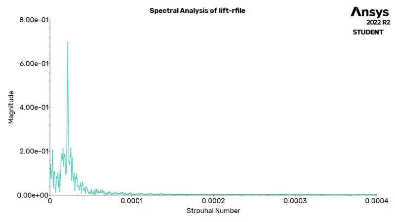
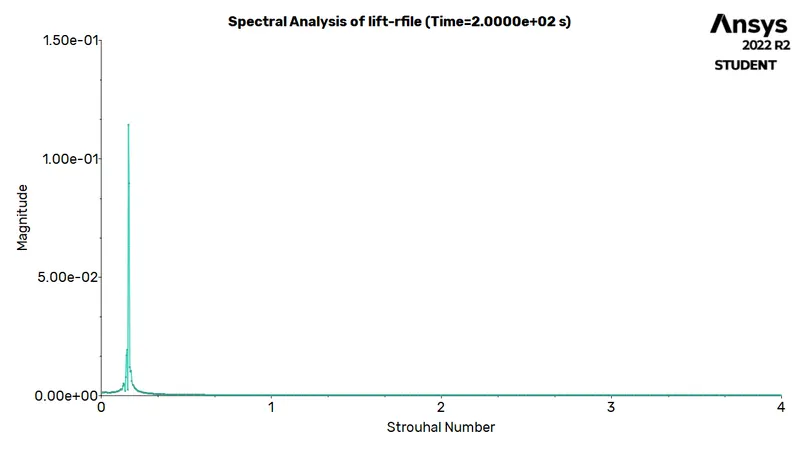
Strouhal Number |
|
`Re 10` |
 |
`-` |
|
`Re 100` |
 |
0.16
|
|
`Re 10^3` |
 |
0.00248
|
|
`Re 10^4` |
 |
0.000232
|
|
`Re 10^5` |
 |
0.0000216
|
|
`Re 100` |
 |
0.15992
|
 |
 |
Conclusion(s):
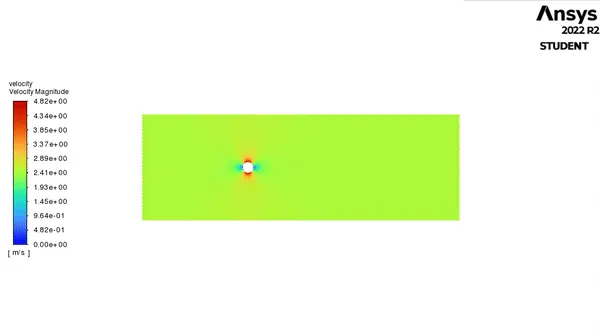
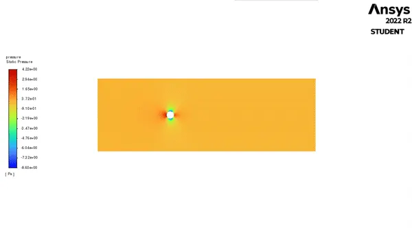
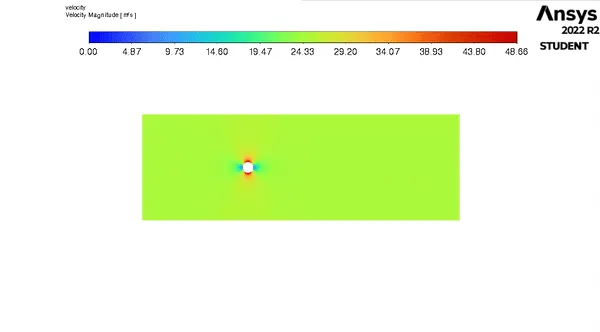
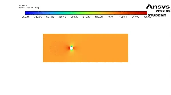
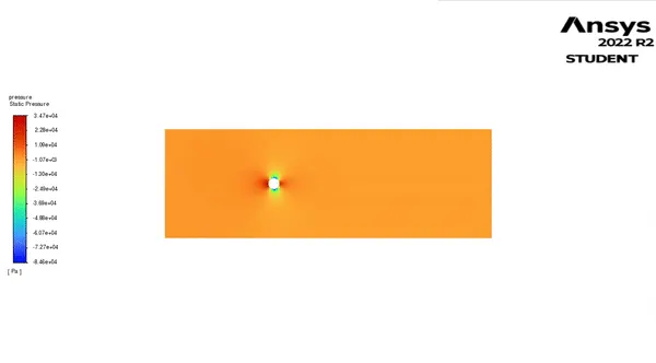
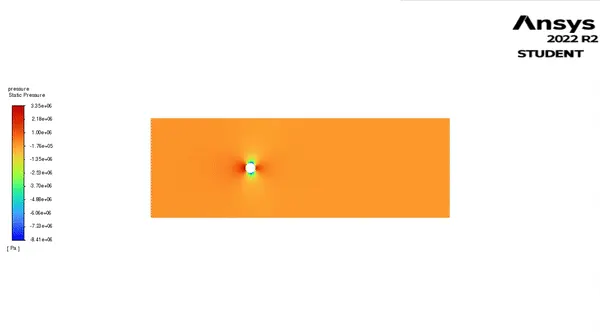
- In all the cases, it is observed that after the flows settles, the pressure in frontal area of the cylinder rises. This is due to the fact that the fluid becomes stagnant at that loaction and in turn, coverts its kinetic energy to pressure energy.
- At low Reynolds number, flow separation does not take place, hence, a streamlined flow over the cylinder wall is observed with little or no changes as the time (here, iterations proceed). Due to this lack of changes, the simulation got converged automatically.
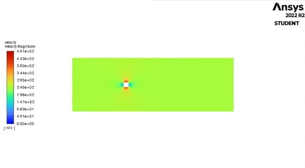
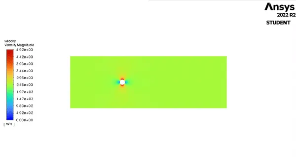
- It is observed that, there is a dramatic rise in velocity, after the fluid strikes the cylinder's frontal region (and this velocity is higher as compared to the free stream velocity. The reason behind this occurence is that, during flow separation, there exists huge energy losses, and consequently, the pressure falls. Due to this drop in pressure, the velocity of fluid rises and hence, sudden influx of fluid at high velocity is observed in this region.
- The alternating nature of the flow detachment (due to which the Karman Vortex Street is formed) causes the pressure to change in an alternating (or oscillating) fashion over the cylinder length. Therefore, the velocity at monitor point, lift and drag coefficient also changes in the same oscillatory manner. The low pressure pockets, generated due to flow separation propagates at the same frequency at which this oscillations occur.
- Although, vortex shedding is a transient phenomenon, it is assumed that the turbulence model takes into account all the unsteadiness occuring in the flow field (due to eddies) and hence, the simulations were performed using steady state solver. However, the separation point of the flow is somewhat downstream, and the results get worse with varying the input parameters. The reason is that the periodic Karman vortex shedding in unsteady in nature, whereas we have forced the solution to be steady. When compared to the solution obtained, from unsteady solver, the dramatic separations are not present and a more refined shedding is spotted.
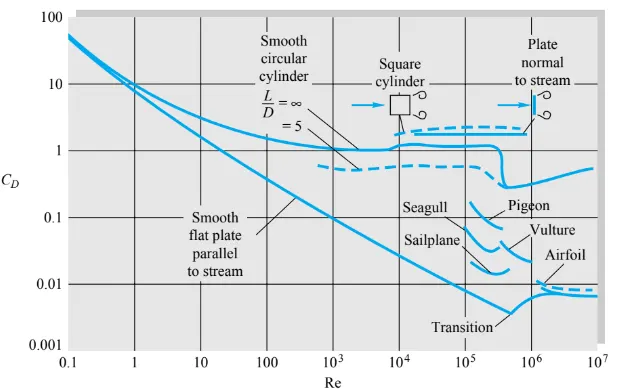
- The results show high degree of coherence with the literature being referred for this problem, and hence, the solution is validated.
Reference(s):
- Introduction to GUI based CFD using Ansys Fluent - Course provided by Skill-Lync
- Ansys Inc.
- Volupe Engineering Software: y+ calculator
- Supporting Material: Numerical simulation of laminar flow past circular cylinder
- Supporting Material: The Sound of Wind: Vortex Shedding and How it Works
- Supporting Material: A-TO-Z GUIDE TO THERMODYNAMICS, HEAT & MASS TRANSFER, AND FLUIDS ENGINEERING
- Supporting Material: Fluid Mechanics - Frank M White
- Supporting Material: Fluid Mechanics: Fundamentals an Applications - Y Cengel and J Cimbala