Week 2 - Flow over a Cylinder.

week 2 challenge:

Simulate the flow over a cylinder and explain the phenomenon of Karman vortex street.

PART-I

1. Simulate the flow with the steady and unsteady case and calculate the Strouhal Number for Re= 100.

PART-II

1. Calculate the coefficient of drag and lift over a cylinder by setting the Reynolds number to 10,100,1000,10000 & 100000. (Run with steady solver)
2. Discuss the effect of Reynolds number on the coefficient of drag. [ Results should be validated with any standard literature and error should be within 5 %]

Expected results:-

1. In both approaches, show that the flow has converged. That is, what quantities or plots need to be looked at to determine that the flow has converged?
2. Plots of the coefficient of drag and lift.
3. Plots to show vortex shedding behind the cylinder.
4. Mention the referred material (Reference Paper or Fluid Mechanics Textbook) at the end of the challenge submission page.

The flow over a 2D cylinder is a very simple flow simulation and has a lot of fluid properties to be monitored while running it. While the flow can be witnessed in real life, It has a specific pattern that forms the Karman Vortex Street. its an oscillation flow phenomenon that can be observed very easily. So let's understand what the Karman Vortex street pattern is all about.

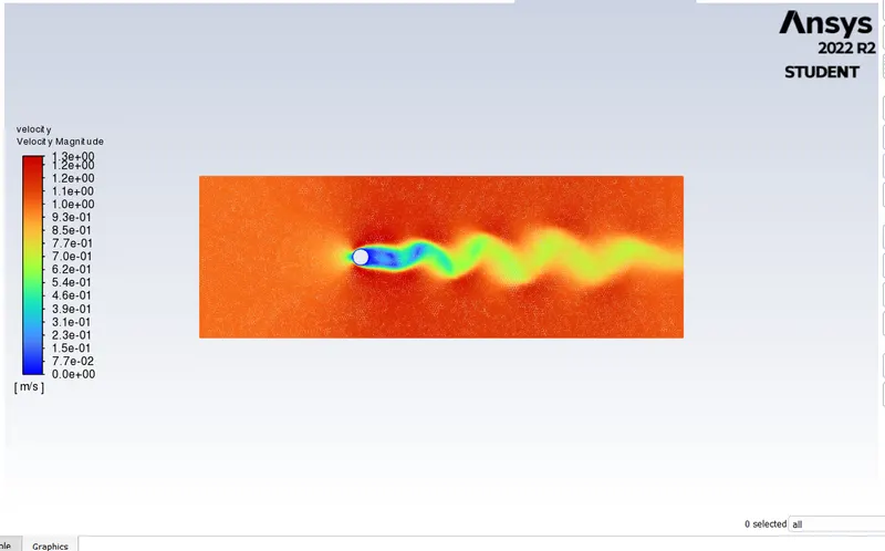
To describe in an informal way the flow created by the motion of a cylinder with constant speed in a fluid at rest. For very small Reynolds numbers, the flow is completely laminar around the cylinder, with no recirculation and no instability. For larger Reynolds numbers, a recirculation zone appears behind the obstacle. More precisely, two eddies with opposite signs appear just behind the cylinder and remain close to it. For larger Reynolds numbers, these eddies are unstable and successively leave the cylinder to propagate in the wake, to form the so-called “Von Karman” vortex street.

solving and modelling:

• Step 1 : Pre-processing/Geometry Creation

1. Launch Ansys workbench. Drag fluent into the work space.
2. draw a circle of radius 2m. and draw a construction line of 20m left and 40 m right from the origin.
3. then draw a rectangle with dimesion of 60x20.
4. Update the project.

• Step 2 : Mesh Generation

1. Open mesh generator in ansys fluent.
2. Selec the faces and name the each face accordingly as inlet, outlet and wall.
3. Generate the default mesh.
4. Edit the element size to 0.25m and update the mesh.
5. Once the mesh is genertaed, we have to change the element type to triangular.
6. generate mesh again.create a inflation layer of 6.
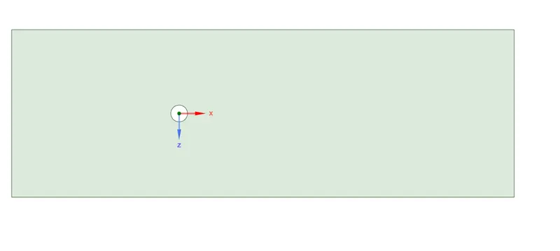
7. close the mesh generator and update the project. Above are some of the examples as to how the vortex pattern forms around a cylinder or any laminar flow at the obstacle in the center. We are going to perform the same phenomenon in ANSYS-FLUENT. First, we are going to create a geometry with a cylinder-like a shape in the middle which will have the same conditions as the cylinder at the center of any fluid flow path. We are going to create this in space claim.

   The following are the tools we used to create the geometry and we have the same after the attempt of creation.

   

   We used line tool to draw with dimensions

   circle - 2m, with circle origin - -20 on X and +40 on X-axis.

   box - 60x20m

   and then used Pull to create a surface from the geometry that looks like

   

   And then move on to Mesh.

   Here we are going to perform mesh and to achieve a very fine Triangular mesh we have to perform certain steps to make sure it is desirable and

   we are to be some different methods and tools to do so. Below are the steps involved in order to do so. This is the former mesh.

   

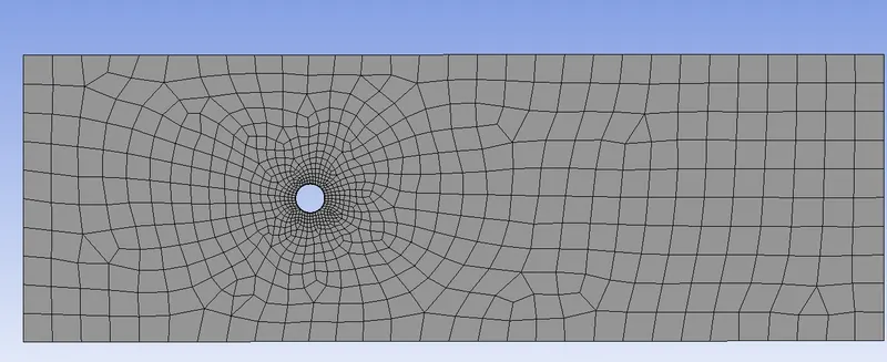
   and that the next steps involve naming selection and making the mesh more fine around the cylinder as well as to the whole computational mesh.

   the following are the tools involved:

   

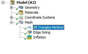
   First, we try to add a method that let us convert quadrilateral mesh to triangle mesh

   

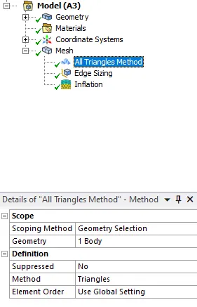
   Though we are going to have undesirable physical simulation at the CFD post with this amount of MESH as we performed beforehand what elements size is suitable for that physical phenomenon.

   So we further tuned it more to finer mesh with an element size of 0.25 and we have

   

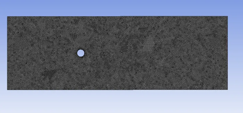
   further, for element sizing, we have a finer cylinder layer where we make it finer by increasing the number of edges by 36 having to be considered as 10 degrees between each other.

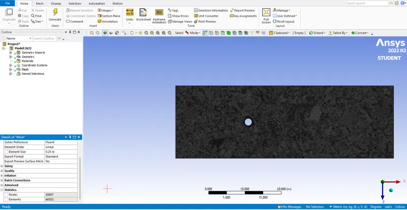
figure of generated mesh.

• Step 3 : Solution Setup

1. Open setup in fluent. The mesh and geometry will be generted. If it doesn't generate then go back to mesh generator and edit accordingly.
2. Click on check mesh button. If the console doesn't show any warning then the mesh is fine.
3. Click on Physics option and select pressure based solver, time as steady, velocity formulation as absolute and clickon Energy button as we need to solve the energy equation.
4. In steady state model select viscous laminar model.
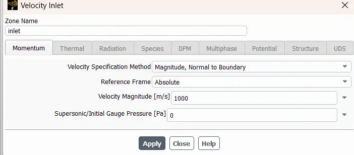
5. Click on solution and input the inlet data for each individual case. Outlet and wall conditions are already setup by fluent solver.
6. Click on definitions and selected Area weighted Average and standard deviation for temperature at the outlet.
7. Click on initialiaze button as the console will run calculation for 10 iterations.
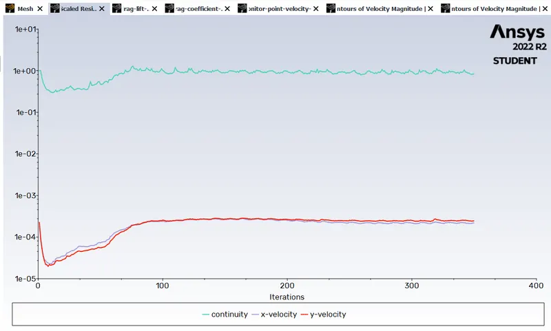
8. Click on Run calculation and set the number of iterations for 350 and hit the calculate button.

PART-I

1. Simulate the flow with the steady and unsteady case and calculate the Strouhal Number for Re= 100.

to calculate the reynolds number we have use the formulaa:

reynolds number=rho*u*d /mu

where rho is the density, u is the velocity of fluid, d is the dimension, mu is the viscosity.

for example.

re=100, we assume the value of viscosity as 0.02, d as 20m

by using the above find the velocity of the fluid.

here velocity=1m/s

the below figure shows the strouhal number for re is 100.

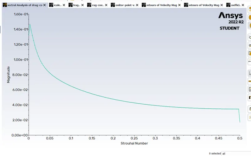
The Strouhal number is defined as St = fstD/U, where fst is the vortex shedding frequency (or the Strouhal frequency) of a body at rest, D is the diameter of the circular cylinder and U is the velocity of the ambient flow.

PART-II

1. Calculate the coefficient of drag and lift over a cylinder by setting the Reynolds number to 10,100,1000,10000 & 100000. (Run with steady solver)
2. Discuss the effect of Reynolds number on the coefficient of drag. [ Results should be validated with any standard literature and error should be within 5 %]

solution 1:

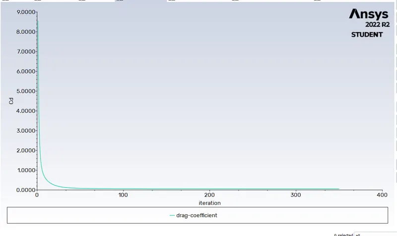
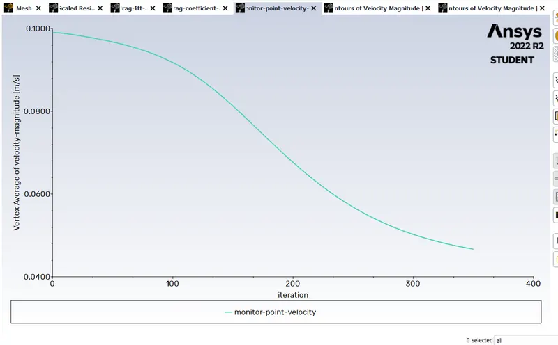
for reynolds number 10.

if we want to set the re.

to calculate the reynolds number we have use the formulaa:

reynolds number=rho*u*d /mu

where rho is the density, u is the velocity of fluid, d is the dimension, mu is the viscosity.

for example.

re=10, we assume the value of viscosity as 0.02, d as 20m

by using the above find the velocity of the fluid.

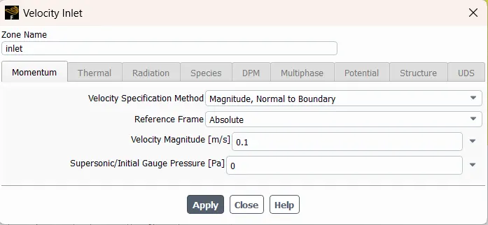
here velocity=0.1m/s

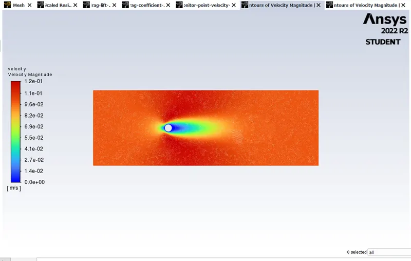
this is the velocity flow over the cylinder with velocity of 0.1m/s

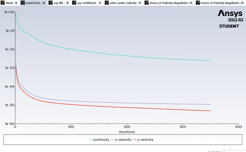
scaled residual vs iteration:

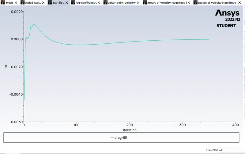
drag lift vs iteration:

drag coefficient vs iteration:

monitor point velocity vs iteration.:

case 2:

to calculate the reynolds number we have use the formulaa:

reynolds number=rho*u*d /mu

where rho is the density, u is the velocity of fluid, d is the dimension, mu is the viscosity.

for example.

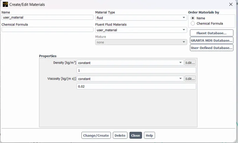
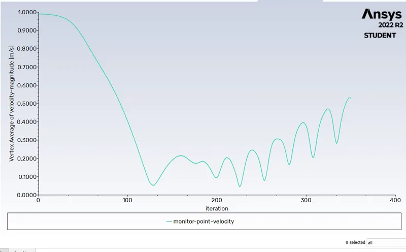
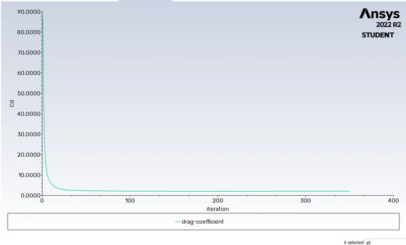
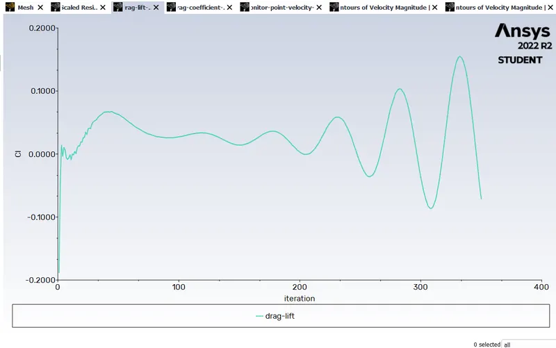
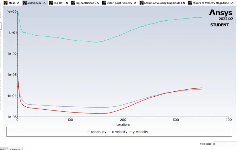
re=100, we assume the value of viscosity as 0.02, d as 20m

by using the above find the velocity of the fluid.

here velocity=1m/s

velocity flow over a cylinder at 1m/s

monitor point velocity vs iteration:

drag coefficient vs iteration:

drag lift vs iteration:

scaled residual vs iteration:

case 3":

to calculate the reynolds number we have use the formulaa:

reynolds number=rho*u*d /mu

where rho is the density, u is the velocity of fluid, d is the dimension, mu is the viscosity.

for example.

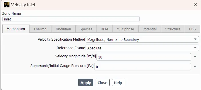
re=1000, we assume the value of viscosity as 0.02, d as 20m

by using the above find the velocity of the fluid.

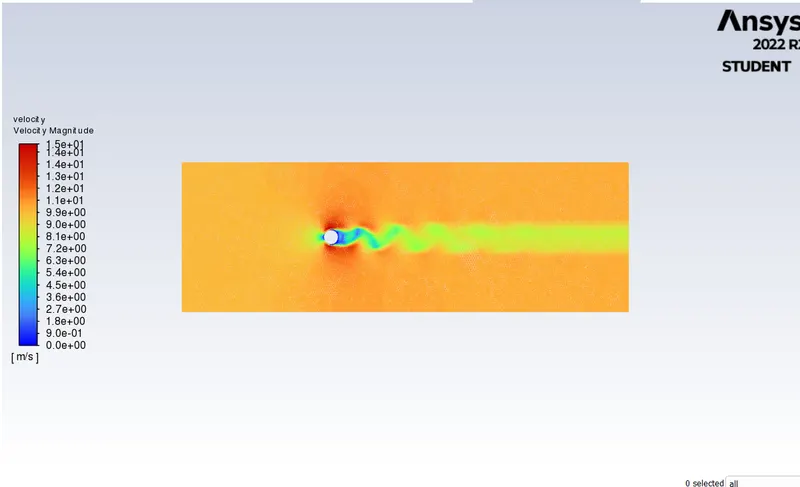
here velocity=10m/s

velocity flow over a cylinder.

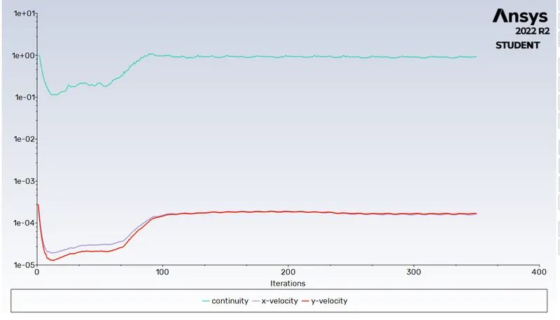
scaled residual vs iteration:

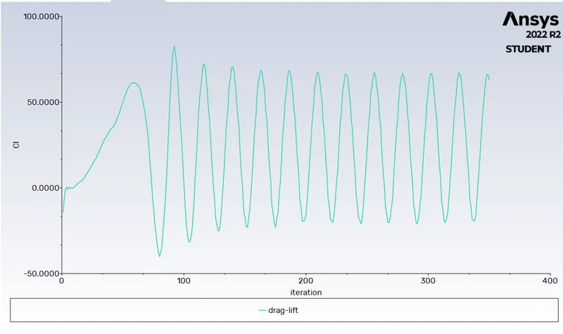
draglift vs iteration:

drag coefficient vs iteration:

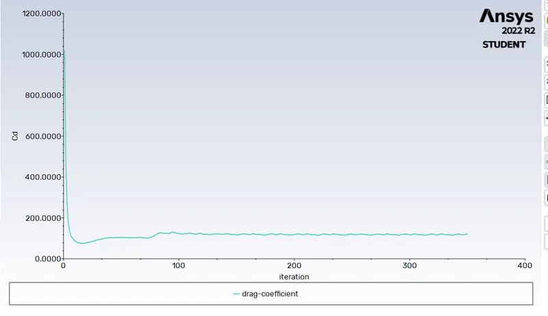
monitor point velocity vs iteration:

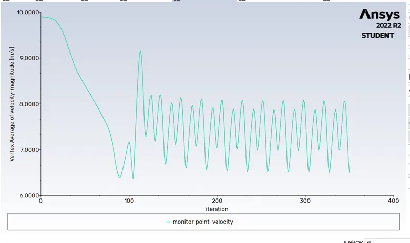
case 4:

to calculate the reynolds number we have use the formulaa:

reynolds number=rho*u*d /mu

where rho is the density, u is the velocity of fluid, d is the dimension, mu is the viscosity.

for example.

re=10000, we assume the value of viscosity as 0.02, d as 20m

by using the above find the velocity of the fluid.

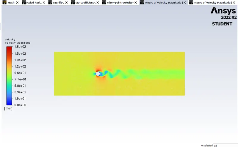
here velocity=100m/s

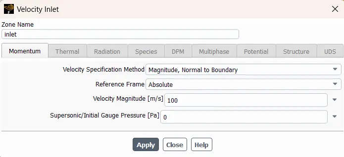
velocity flow:

scaled residual vs iteration:

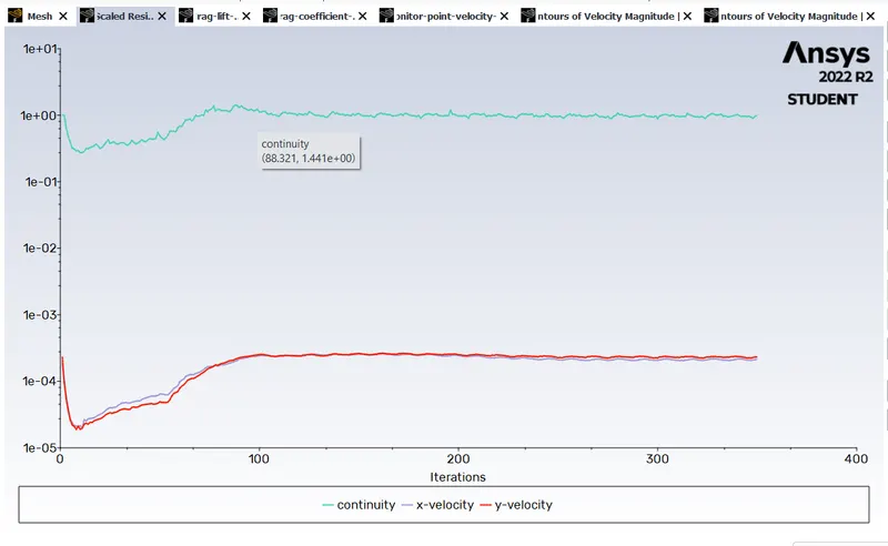
drag coefficient vs iteration:

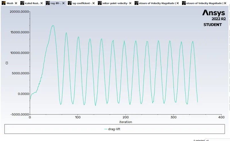
drag coefficient vs iteration:

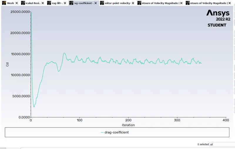
monitor poiint velocity vs iteration:

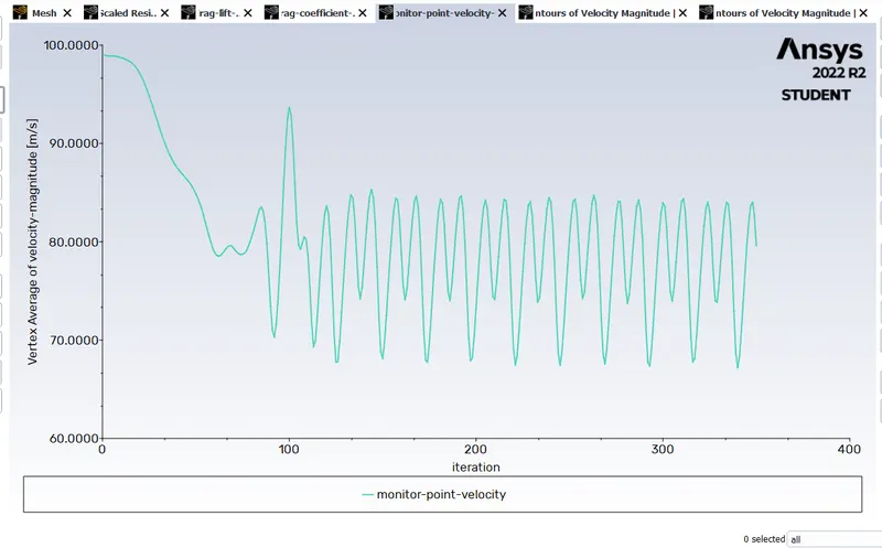
case 5:

to calculate the reynolds number we have use the formulaa:

reynolds number=rho*u*d /mu

where rho is the density, u is the velocity of fluid, d is the dimension, mu is the viscosity.

for example.

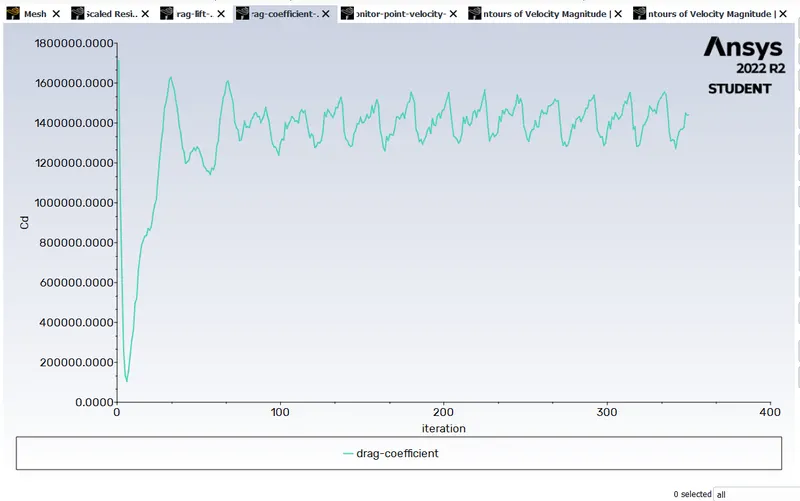
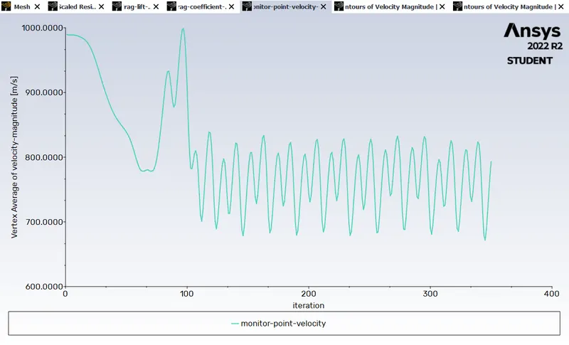
re=100000, we assume the value of viscosity as 0.02, d as 20m

by using the above find the velocity of the fluid.

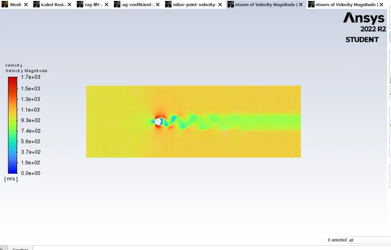
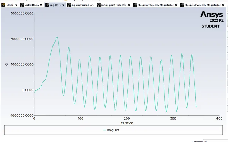
here velocity=1000m/s

velocity flow over cyclinder.

scaled residual vs iteration:

drag lift vs iteration:

drag coefficient vs iteration:

monitor point vs iteration:

conclusion:

from the above figure, that is shown th value of scaled residual drag coefficient, lift , velocity flow vs iteration for the re of 10,100,1000,10000,100000.

by changing the value of velocity we obtain the reynolds number ie.0.1,1,10,100,1000 for re of 10,100,1000,1000,100000

Solution 2:

The effect of Reynolds number on the coefficient of drag and Lift done by aerodynamic experimentation of an airfoil with gurney flap

Lift coefficient decreases rapidly and drag coefficient increases rapidly when Reynolds number is decreased below critical range. This occurs due to a change in flow pattern near the Gurney flap at low Reynolds numbers.

A computational investigation on the effects of Reynolds number on the aerodynamics of NACA0012 airfoil without and with Gurney flap of the height of 3% airfoil chord has been carried out. ANSYS FLUENT commercial CFD code with one-equation Spalart-Allmaras turbulence model is used for the six Reynolds numbers varying from 3.0 × 10⁵ to 3.0 × 10⁴. From this investigation, the following major conclusions are drawn.

(1)Reynolds number plays a very major role in the airfoil aerodynamics for the NACA0012 airfoil without and with Gurney flap. Lift decreases and drag increases when Reynolds number is decreased.

(2)For the airfoil with GF, Reynolds number has adverse effects on lift coefficient, while the drag coefficient of the airfoil with GF has some beneficial effects compared to the airfoil without GF.

(3)For high Reynolds number above critical range, decrease in Cl and Cd increase in are negligible.

(4)As the Reynolds number is decreased below the critical Reynolds number range, Cl decreases and Cd increases at a very steep rate and the performance degrade rapidly.

(5)For lower Reynolds numbers, the two vortices behind the Gurney flap vanish. The Gurney flap seems to increase the effective camber of the airfoil, causing a negative zero-lift angle and reduced stall angle.

research paper::

in the research paper , it has been shown that 2d and 3d flow over a cylinder in different laminar regimes.

pressure based finite volume material with the time accurate computation of incompressible fluid of second order convective flux discretization is used.

cross flow normal to the axis of a stationary circular cylinder and associated heat and mass transfer.

experimental data is compared with the numerical computation data. it shows the new alue.

it is well known as karman vortex street.

in case of streamline flow over cylinder.

reynolds number=rho*u*d /mu

where rho is the density, u is the velocity of fluid, d is the dimension, mu is the viscosity.

for laminar flow the re is between 1 to 100 and greater then the is turbulant.

characteristic of flow past over a circular cylinder:

zdravkovich, in his excellent monograph.

since 1938, he collected all the experimental, theoretical , and analytical simulation data on a flow over a cylinder and he classified it into five differnent flow regimes. this is shown in the below figure.

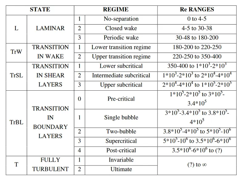
all the computation are done using pressure based finite volume navier stokes algorithm(RANDs3d) for time accurate prediction of flow.

result:

in case of l1 and l2 regime , where the flow is steady . the present computationare limited to 2 d flow only.

l3 regime of periodic vertoex shedding for re upto 200, the flow structure in the periodic wake region.

computation upto 200 re,, are therefore 2d flow and it is compared with measurement data reported in the literature of strouhal frequency , circumferential variation of time, average surface pressure and skin friction and rms values of lift and drag coefficient.

beyond the critical value re of 180-200 , the measurement as well as numerical simulation data demonstrate a suspect of the 2d wake behind the cylinder to 3d floquent instability.

conclusion::

upto re 200 , the 2d computational reports agree reasonably well with the accurate measurement data for the strouhal frequency, the base presure coefficient and the mean drag coefficient.

however, beyond the critical re180 . gross discrepancies have been observed between 2d result and measured data.

referance:

https://www.sciencedirect.com/science/article/pii/S0307904X08000243

Effect of Reynolds Number on Aerodynamics of Airfoil with Gurney Flap (hindawi.com)