Week 2 - Flow over a Cylinder.

AIM:

To simulate the flow over a cylinder and explain the phenomenon of Karman vortex street. Understanding the vortex shedding for different Reynolds numbers by changing the inlet velocities accordingly. Create a monitor point behind the cylinder at a distance 4 times the diameter which can be used to calculate and analyze the vortex shedding.

OBJECTIVE:

1. Simulate the flow with the steady and unsteady case and calculate the Strouhal Number for Re= 100

2. Calculate the coefficient of drag and lift over a cylinder by setting the Reynolds number to 10,100,1000,10000 & 100000. (Run with steady solver)

2. Discuss the effect of Reynolds number on the coefficient of drag. [ Results should be validated with any standard literature and error should be within 5 %]

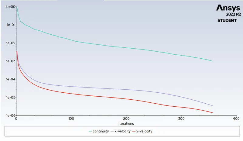
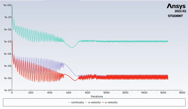
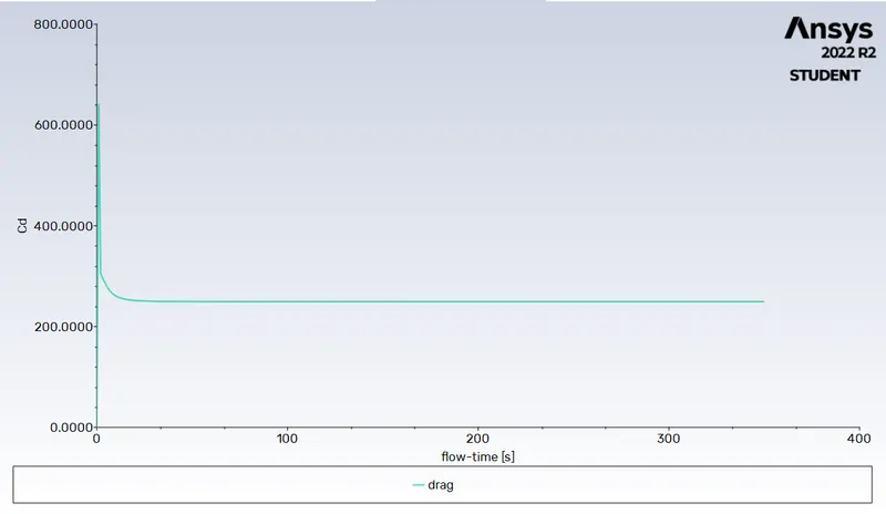
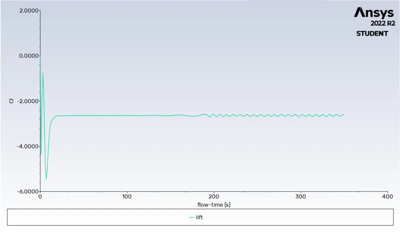
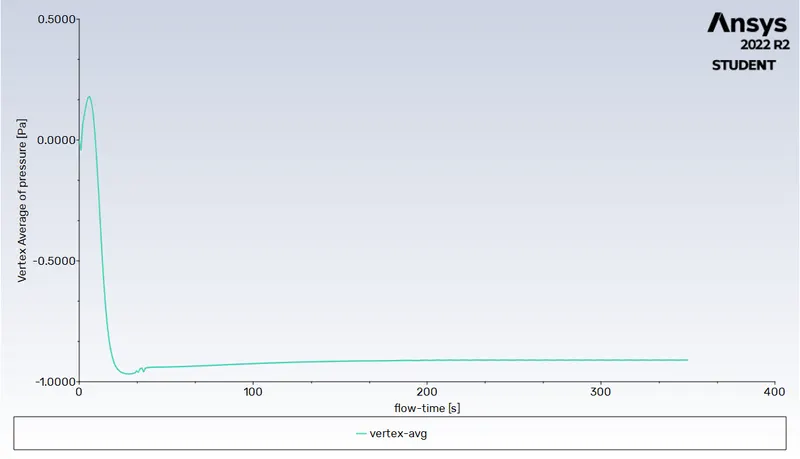
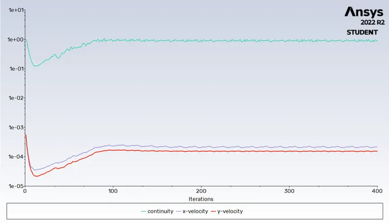
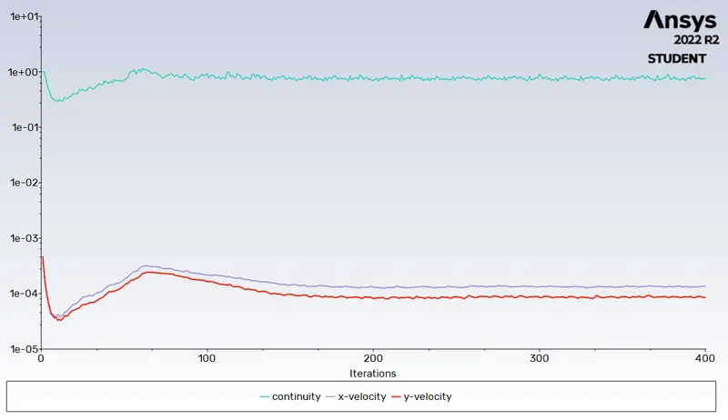
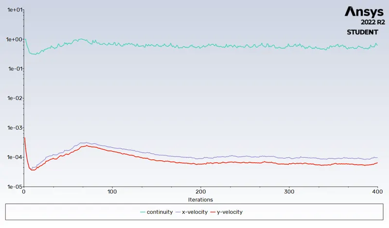
3. In both approaches, show that the flow has converged. That is, what quantities or plots need to be looked at to determine that the flow has converged?

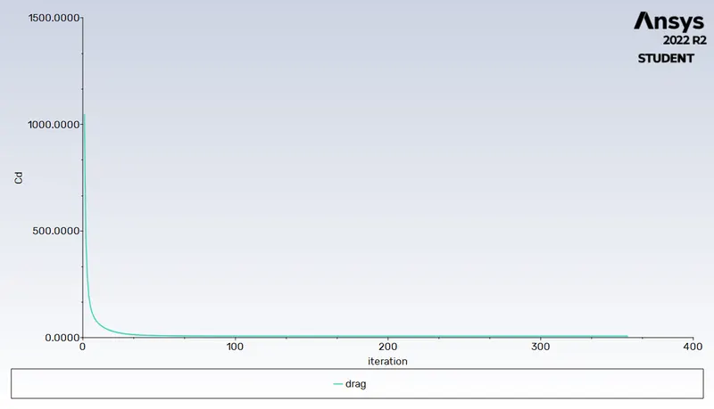
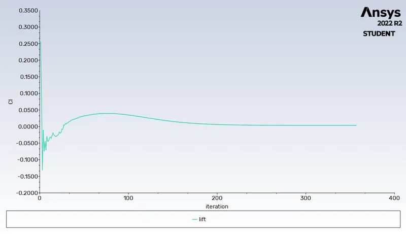
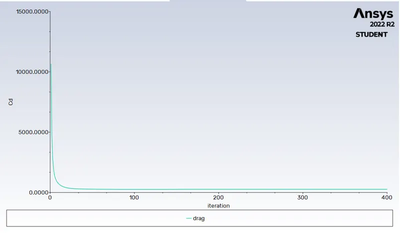
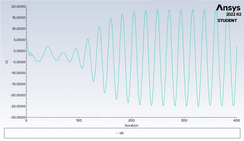
4. Plots of the coefficient of drag and lift.

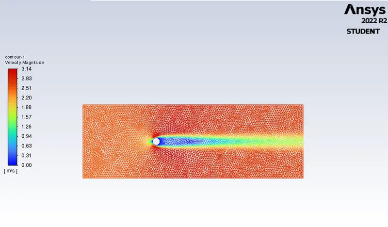
5. Plots to show vortex shedding behind the cylinder.

6. Mention the preferred material at the end of the challenge submission page.

Strouhal number:

In dimensional analysis, the Strouhal number is a dimensionless number describing oscillating flow mechanisms.

For large Strouhal numbers (order of 1), viscosity dominates fluid flow, resulting in a collective oscillating movement of the fluid "plug". For low Strouhal numbers (order of 10⁻⁴ and below), the high-speed, quasi-steady-state portion of the movement dominates the oscillation. Oscillation at intermediate Strouhal numbers is characterized by the buildup and rapidly subsequent shedding of vortices.

The Strouhal number is often given as

`S_t=(fD)/(U')`

Where,

f= frequency of vortex shedding

D= characteristic diameter of the cylinder

U'= fluid flow velocity

A brief explanation to solve the flow over a cylinder.

1. Geometry

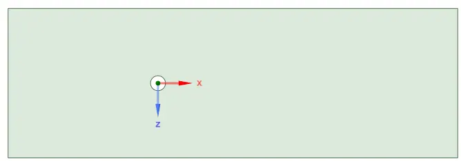
Creating the geometry by sketching using the line and circle command, circle diameter of 2m and the dimensions having 20X60m and the circle is placed 20m from the inlet.

2.Mesh

After the geometry is loaded we should mesh it and here I used 0.19m as elemental size

But in the meshing nodes, the shape is more quadrilateral than the triangle so we should this by changing the method to the triangle in the insert option

After changing the node's shape into triangles we should improve the mesh around the cylinder by sizing in the mesh which is used to control precisely the mesh.

Then we should add inflation which is used to create body-fitted mesh.

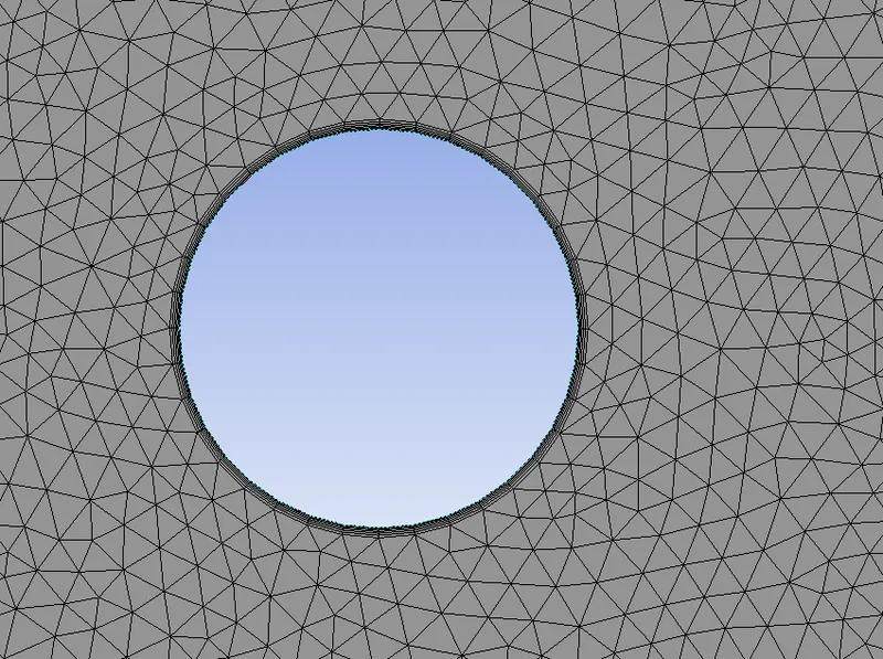
And we should name the boundaries as given below

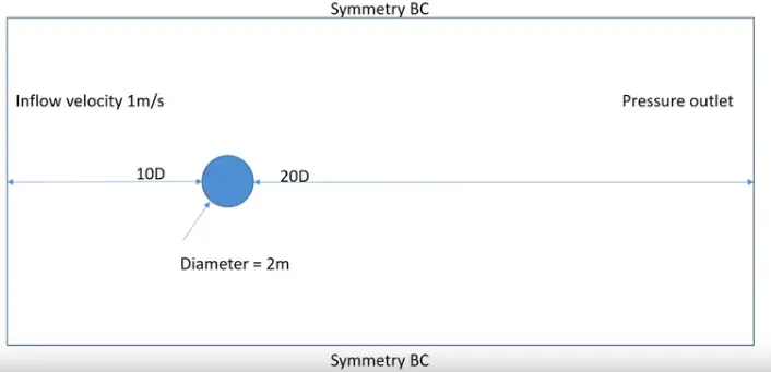
where cylinder edge is named as wall.

3.Setting up Ansys fluent

Before opening the set up we should update the mesh. Then we should change the viscous flow to laminar

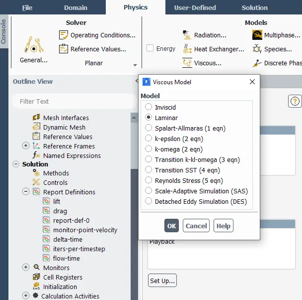
Open Materials and create a fluid that is to be used for the simulation for this case, it is air and also inputs the density and kinematic viscosity values.

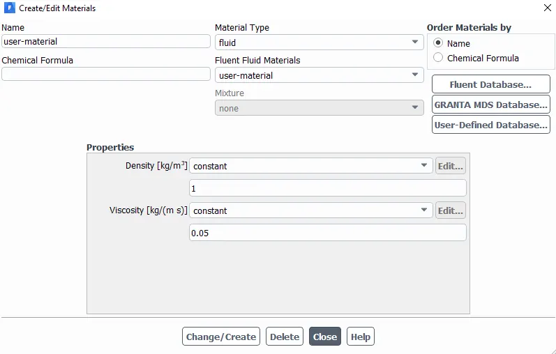
Open Zones and input the inlet velocity as per the reynolds number and check if the fluid is updated.

Update the reference values which is located inside set up at the right-hand side.

Fluent details/procedure:

a. laminar model

b. fluid: Air

c. Method of discretization: Simple

d. Density/kinematic viscosity: 1/0.05

e. Creating a monitor point behind the cylinder by selecting point under surfaces in the results bar.

f. After creating the monitor point, create reports/plots for drag, lift, velocity wrt cylinder.

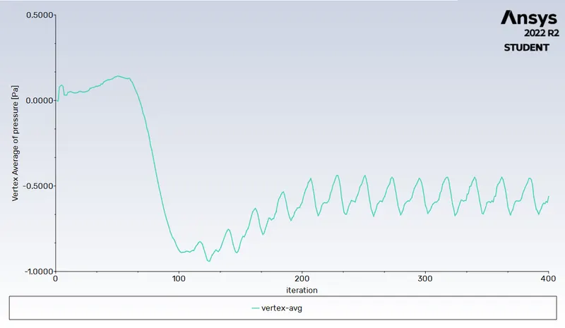
g. Create plots for the velocity at the monitor point to analyze the vortex shedding.

h. Use hybrid initialization for steady-state and standard for transient state simulations.

(i) Simulate the flow with the steady case for Re=10 and velocity 0.25m/s.

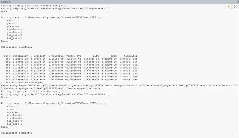
Residuals:

Drag-coefficient:

lift-coefficient:

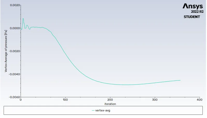
Vertex-avg:

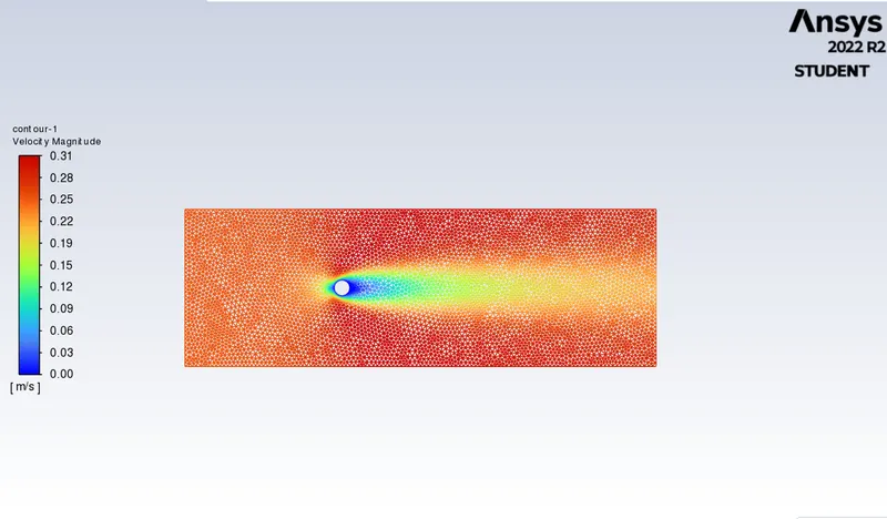
Velocity contour:

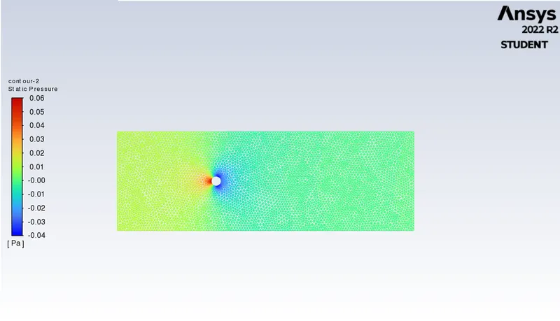
pressure contour:

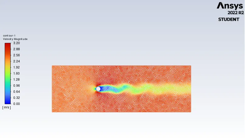
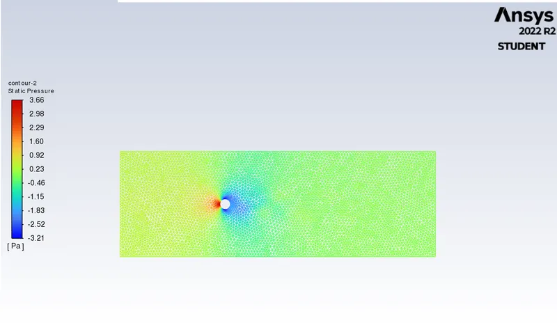
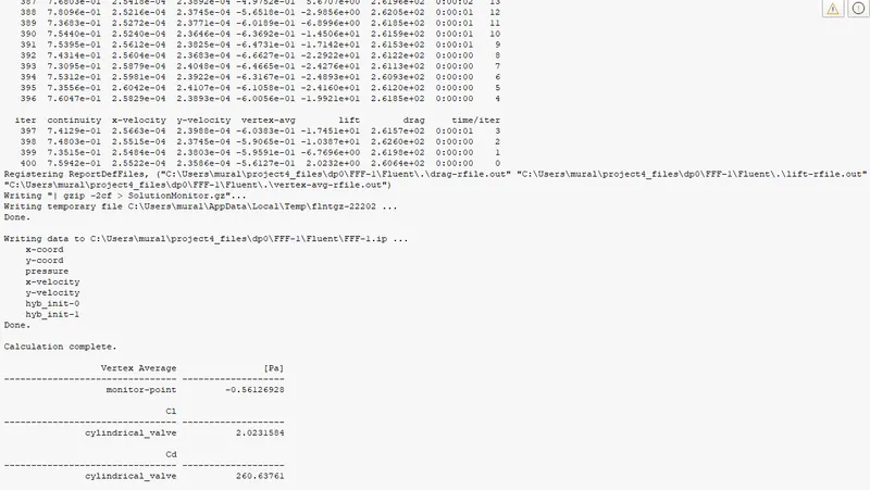
Simulate the flow with the steady case and calculate the Strouhal number for Re=100 and velocity 2.5m/s.

Residuals:

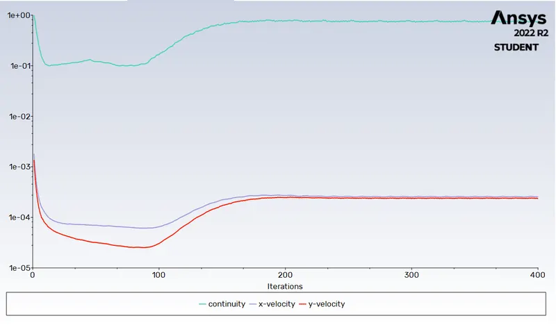
Drag-coefficient:

lift-coefficient:

vertex-avg:

velocity-contour:

pressure-contour:

computed:

Transient state: Re=100

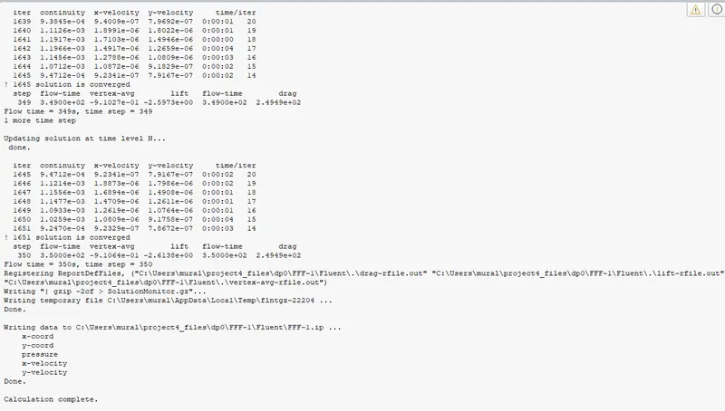
residuals:

drag-coefficient:

lift-coefficient:

vertex-avg:

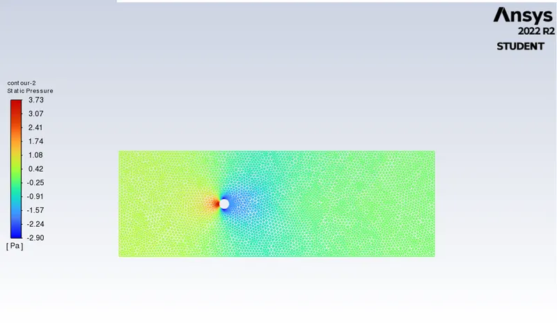
velocity contour:

pressure contour:

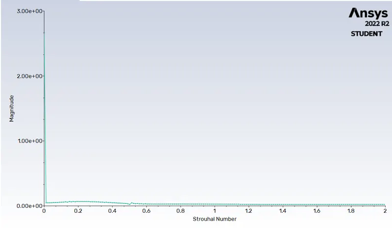
strohal number: Re=100

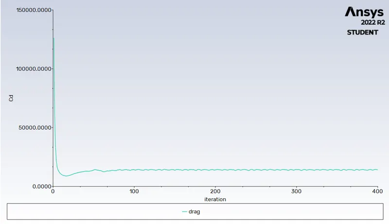
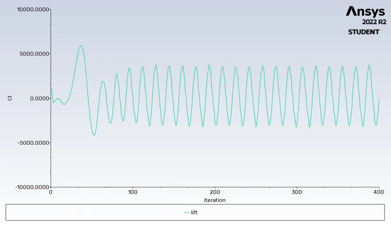
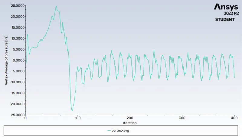
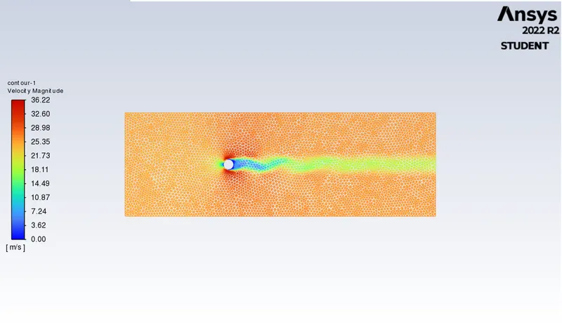
Simulate the flow with the steady case for Re=1000 and velocity 25m/s.

residuals:

drag-coefficient:

lift-coefficient:

vertex-avg:

velocity contour:

pressure contour:

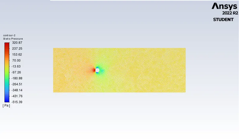
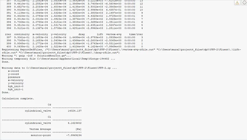
computed:

Simulate the flow with the steady case for Re=10000 and velocity 250m/s.

residuals:

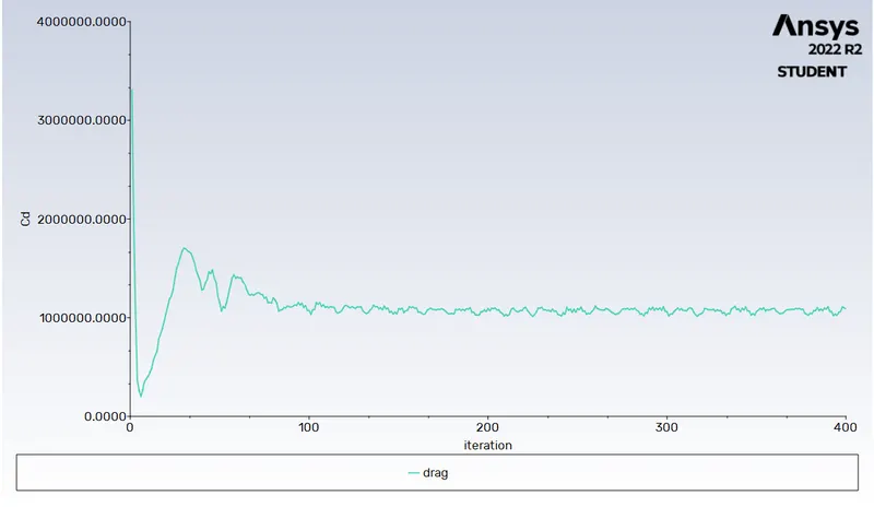
drag-coefficient:

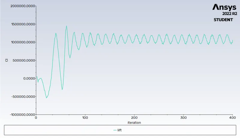
lift-coefficient:

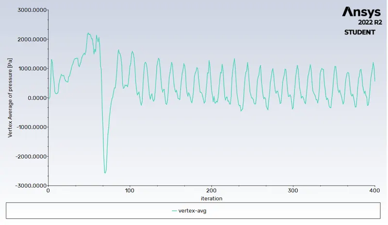
vertex-avg:

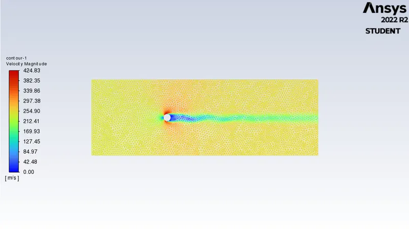
velocity contour:

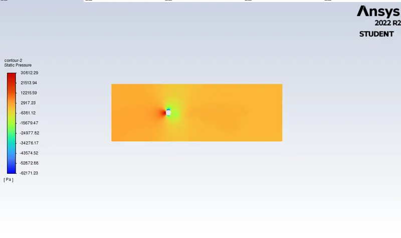
pressure contour:

computed:

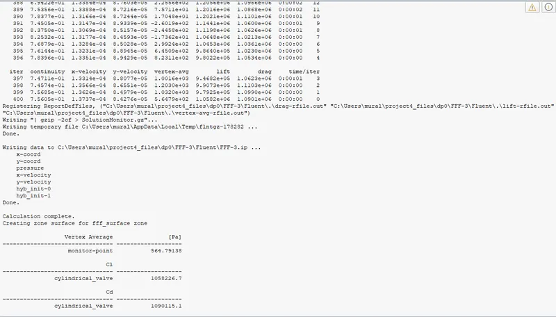
Simulate the flow with the steady case for Re=100000 and velocity 2500m/s.

residuals:

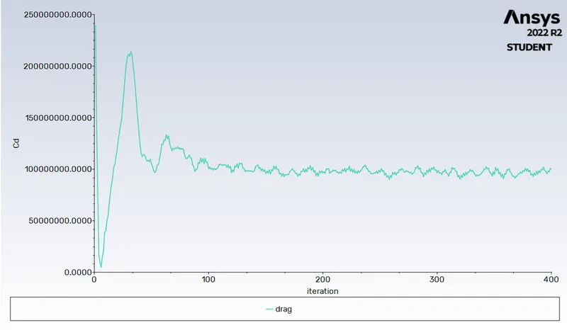
drag-coefficient:

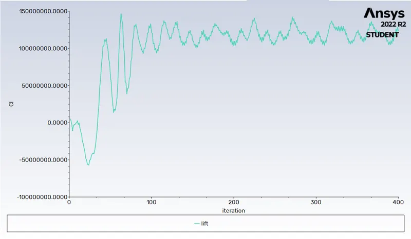
lift-coefficient:

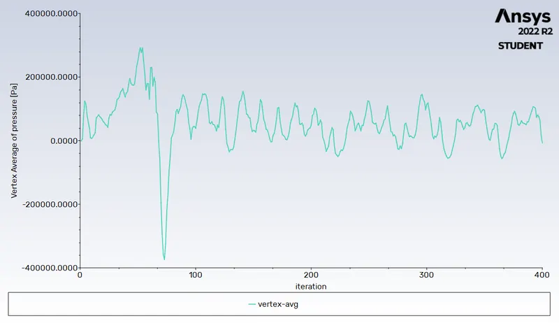
vertex-avg:

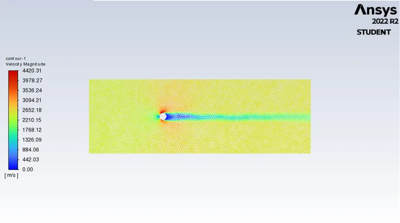
velocity contour:

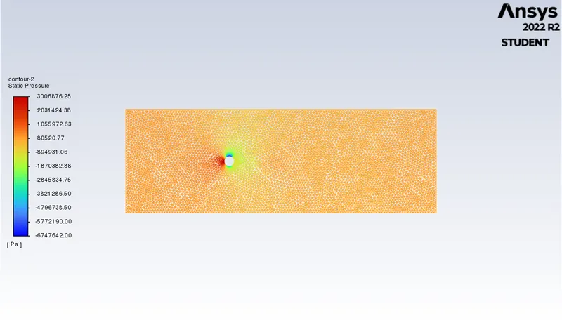
pressure contour:

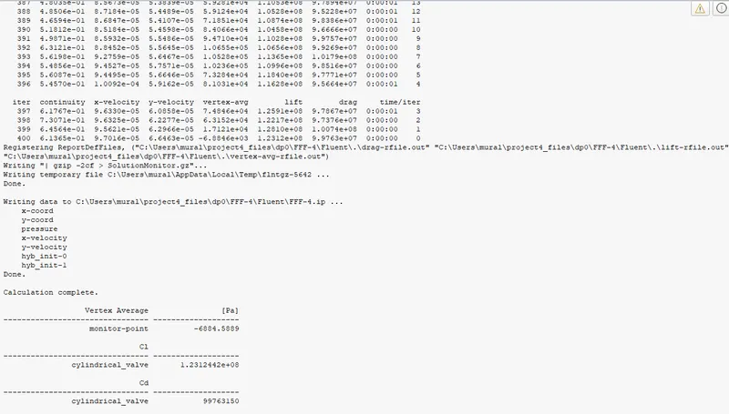
computed:

Result:

Drag and lift coefficient for different Re

Re	Cd	CL
10	130.332	1.00155
100	260.637	2.0231
1000	14024.137	4.16236
10000	1090115.1	1058226.7
100000	99763150	1.23124

Conclusions:

• flow over a cylinder is simulated for both Steady and unsteady cases with Re=100, and with the results generated the phenomena of Von Karman Vortex Street are also observed.
• five different simulations i.e (Re = 10,100,1000,10000,100000) are simulated to observe the behavior of the drag and lift coefficients by changing the Reynolds number.
• In order to observe the behavior of the drag coefficients for the simulations, the velocity of the flow is varied to change the Reynolds number and the rest of the parameters are kept constant.
• Necessary plots are plotted in order to observe that the flow is converged and the vortex shedding is happening.
• Contours are generated in order to observe the flow over a cylinder.
• By plotting Power Spectral Density vs Frequency, the Strouhal number is calculated.